9.4. User-Defined Output
BEGIN FILTER <string>filter_name
  ACOEFF = <real_list>a_coeff
  BCOEFF = <real_list>b_coeff
  INTERPOLATION TIME STEP = <real>ts
END [FILTER <string>filter_name]

BEGIN USER OUTPUT
  # mesh-entity set commands
  NODE SET|NODESET = <string list>nodelist_names
  SURFACE = <string list>surface_names
  BLOCK = <string list>block_names
  ASSEMBLY = <string list>assembly_names
  INCLUDE ALL BLOCKS
  REMOVE NODE SET = <string list>nodelist_names
  REMOVE SURFACE = <string list> surface_names
  REMOVE BLOCK = <string list>block_names
  #
  # compute result commands
  PROCESS ELEMENTS = ACTIVE_ONLY|INACTIVE_ONLY|ALL(ACTIVE_ONLY)
  COMPUTE {GLOBAL} <string>result_var_name
    AS {SUM|MAX|MIN|MAX ABSOLUTE VALUE|L2NORM|VARIANCE}
    OF {NODAL|ELEMENT|FACE} <string>source_var_name
  COMPUTE {GLOBAL} <string>result_var_name
    AS AVERAGE
    OF {NODAL|ELEMENT|FACE} <string>source_var_name
    [WEIGHTED BY <string>weight_var_name]
  COMPUTE {GLOBAL|NODAL|ELEMENT} <string>result_var_name
    AS NONLOCAL AVERAGE
    OF {NODAL|ELEMENT} <string>source_var_name
    OVER DOMAIN DEFINED BY RADIUS <real>r
    [AND POINT <real>x <real>y <real>z]
  COMPUTE {GLOBAL} <string>result_var_name
    AS {VOLUME INTEGRAL|SURFACE INTEGRAL}
    OF {NODAL|ELEMENT} <string>source_var_name
  COMPUTE {GLOBAL} <string>result_var_name
    AS CLOSEST DISTANCE TO <string> mesh_entity_name SEARCH {KDTREE_NODE_FACE|NODE_FACE|NODE_NODE|MIXED}
  COMPUTE {GLOBAL} <string>result_var_name
    AS FURTHEST DISTANCE TO <string> mesh_entity_name
  COMPUTE {GLOBAL} <string>result_var_name
    AS MAX NORMAL|OPPOSING GAP BETWEEN <string> mesh_entity_name
  COMPUTE {GLOBAL} <string>result_var_name
    AS SURFACE INTEGRAL OF {ELEMENT} {ELEMENT_LOCAL_FORCE}
    IN DIRECTION <real>dx <real>dy <real>dz
  COMPUTE GLOBAL <string>result_var_name AS
    INTERNAL REACTION [VECTOR|SHEAR|TRANSVERSE|NORMAL(VECTOR)]
    [AT POINT <real>px <real>py <real>pz]
    [IN DIRECTION <real>dx <real>dy <real>dz]
  COMPUTE GLOBAL <string>result_var_name AS
    INTERNAL MOMENT [VECTOR|TRANSVERSE|NORMAL(VECTOR)]
    [AT POINT <real>px <real>py <real>pz]
    [IN DIRECTION <real>dx <real>dy <real>dz]
  COMPUTE GLOBAL <string>result_var_name AS INTERPOLATION
    OF NODAL <string>source_var_name
    AT POINT <real>x <real>y <real>z

  COMPUTE {GLOBAL|NODAL|ELEMENT|FACE} <string>result_var_name
    AS FUNCTION <string>function_name
  COMPUTE {GLOBAL} <string>result_var_name
    FROM EXPRESSION "<string>expression"
  COMPUTE {GLOBAL} <string>result_var_name
    AS {INTEGRAL OVER TIME|LOG|EXP|MAGNITUDE} OF {GLOBAL}
    <string>source_var_name

  COMPUTE {NODAL} <string>result_var_name AS
    {MAX OVER TIME|MIN OVER TIME|ABSOLUTE VALUE MAX OVER
    TIME|AVERAGE OVER TIME|STANDARD DEVIATION OVER TIME|
    LOG|EXP} OF {NODAL} <string>source_var_name
  COMPUTE {NODAL} <string>result_var_name AS
    {ROLLING AVERAGE OVER TIME} OF {NODAL} <string>source_var_name
    WINDOW WIDTH <real> window_width
    COMPUTE {NODAL} <string>result_var_name AS !explicit_mini!
    END STEP VALUE OF {NODAL} {VELOCITY}

  COMPUTE {ELEMENT} <string>result_var_name AS
    {MAX OVER TIME|MIN OVER TIME|ABSOLUTE VALUE MAX OVER TIME|
    AVERAGE OVER TIME|STANDARD DEVIATION OVER TIME}
    OF {ELEMENT} <string>source_var_name
  COMPUTE {ELEMENT} <string>result_var_name AS
    {MAX|MIN|VOLUME WEIGHTED AVERAGE|
     UNWEIGHTED AVERAGE|AVERAGE|LOG|EXP} OF {ELEMENT} <string>source_var_name
  COMPUTE {ELEMENT|FACE} <string>result_var_name AS
    {MAX|MIN} OF {NODAL} <string>source_var_name
  COMPUTE {ELEMENT|FACE} <string>result_var_name AS
    AVERAGE OF {NODAL} <string>source_var_name
    [WEIGHTED BY <string>weight_var_name]


  #
  # user subroutine commands
  NODE SET SUBROUTINE = <string>subroutine_name |
    SURFACE SUBROUTINE = <string>subroutine_name |
    ELEMENT BLOCK SUBROUTINE = <string>subroutine_name
  SUBROUTINE DEBUGGING OFF | SUBROUTINE DEBUGGING ON
  SUBROUTINE REAL PARAMETER: <string>param_name
    = <real>param_value
  SUBROUTINE INTEGER PARAMETER: <string>param_name
    = <integer>param_value
  SUBROUTINE STRING PARAMETER: <string>param_name
    = <string>param_value
  #
  # copy command
  COPY ELEMENT VARIABLE <string>ev_name
    TO NODAL VARIABLE <string>nv_name
  COPY {MAX|SUM|WEIGHTED SUM} ELEMENT VARIABLE <string>ev_name
    TO NODAL VARIABLE <string>nv_name
  #
  # extrapolate command
  EXTRAPOLATE ELEMENT VARIABLE <string>ev_name to NODAL VARIABLE
    <string>nv_name
  EXTRAPOLATE PROJECTION TYPE = <string>projection_type
    {CONSISTENT|ROW_SUM_LUMPED|PROPORTIONAL_LUMPED} (CONSISTENT)
  LINEAR SOLVER = <string>solver_name (DEFAULT_FETI_SOLVER)
  #
  # variable transformation command
  TRANSFORM {NODAL|ELEMENT} VARIABLE <string>variable_name
    TO COORDINATE SYSTEM <string>coord_sys_name
    AS <string> transformed_name
    [ FROM {MODEL|CURRENT}(CURRENT) COORDINATES ]
  # nonlocal averaging with additional options
  BEGIN NONLOCAL AVERAGE <string>name
    SOURCE VARIABLE = NODAL|ELEMENT <string>variable_name
    TARGET VARIABLE = NODAL|ELEMENT|GLOBAL <string>variable_name
    RADIUS = <real>radius_value
    POINT = <real>x <real>y <real>z
    #options only for nodal nonlocal averaging
    NUMBER OF RINGS = <int>num_rings
    DISTANCE WEIGHTING FUNCTION = <string>function_name
    DISTANCE ALGORITHM = EUCLIDEAN_DISTANCE |
                         GRAPH_DISTANCE | EUCLIDEAN_GRAPH
    WEIGHTING VARIABLE = <string>nodal_weighting_variable_name
    PRINT DEBUG INFORMATION FOR NODE = <int>node_id
    #option only for element nonlocal averaging
    SAMPLE POINTS IN SPHERE AT RADIAL INCREMENT
          <real>increment AND ANGLE <real>angle
    #option only for computing a global target variable
    OUTPUT IN LOCAL COORDINATE SYSTEM \#
          <optional_string> COORDINATE_SYSTEM_NAME
  END
  #
  # data filtering
  FILTER <string>new_var FROM {GLOBAL|NODAL|ELEMENT|FACE}
    <string>source_var USING <string>filter_name
  #
  # compute for element death
  COMPUTE AT EVERY STEP !explicit_mini!
  #
  # fine-grained control of when output is computed
  COMPUTE AT {HEARTBEAT|HISTORY|RESULTS} OUTPUT STEPS \#
        DATABASE NAME <string>database_name
  #
  # additional command
  ACTIVE PERIODS = <string list>period_names
  INACTIVE PERIODS = <string list>period_names
END [USER OUTPUT]
Warning
A new USER OUTPUT block should be created in the input deck when using a different type of command line, since user output operations are order-dependent. If placed in the same USER OUTPUT block, the order the commands are processed may be incorrect, causing errors in computed results.
The USER OUTPUT command block enables the user to generate specialized output information which is derived from analysis results such as element stresses, displacements, and velocities. USER OUTPUT post-processes analysis results in situ, as the code is running, to produce a reduced set of specialized output information. The USER OUTPUT command block offers an alternative to writing out large quantities of data and then post-processing them with an external code to produce customized output results.
As an example, the USER OUTPUT command block could be used to sum the contact forces in a particular global axis direction, on a certain surface in the mesh, to yield a net resultant contact force on that surface. In this instance, USER OUTPUT would reduce a potentially large set of detailed contact data to a single, meaningful value for a surface (or set of surfaces).
!explicit!
In an explicit analysis, the USER OUTPUT command block may also be used to define a user element failure criterion. In this case, the COMPUTE AT EVERY STEP command must be used to ensure that the variable is computed at every time step. See Section 9.4.9 on element death for additional details.
There are several options for calculating user-defined quantities:
ComputeA single command line in the command block is used to compute reductions of variables on subsets of the mesh. This option makes use of one of theCOMPUTEresult command lines. For instance, the above example of the contact force is a case where we can accomplish the desired result by using theCOMPUTE GLOBALcommand line.User subroutineThe command block specifies a user subroutine to run immediately preceding output to calculate any desired variable. This option makes use of aNODESET,SURFACE, orELEMENT BLOCK SUBROUTINEcommand line.CopyThere is an option to copy an element variable for an element to the nodes associated with the element, via theCOPY ELEMENT VARIABLEcommand line, made available primarily for creating results files for some of the post-processing tools used with Sierra/SM.
Only one of these three options may be used in a given USER OUTPUT command block.
For the compute result option, a user-defined variable is automatically generated. This user-defined variable is given whatever name the user selects for results_var_name in the above specification for any of the three compute result command lines. Parenthesis syntax (Section 9.1) may be used to define reductions on integration points or components of a variable. By default, a reduction operation operates on each integration point. For example, if the compute global command was used to average values of element stress it would average the values of stress at all integration points of all elements. If the command was used to average stress(:,1), the result would only be the average of stress on the first integration points.
If the user subroutine or copy option is used, the user will need to define some type of user variable with the USER VARIABLE command block described in Section 10.2.4.
User-defined variables, whether they are generated via the compute result option or the USER VARIABLE command block, are not automatically written to a results or history file. If the user wants to output any user-defined variables, these variables must be referenced in a results or history output specification (see Section 9.3.1 and Section 9.7, which describe the output of variables to results files and history files, respectively).
The USER OUTPUT command block contains five groups of commands—mesh-entity set, compute result, user subroutine, copy, and compute for element death. Each of these command groups is independent of the others. In addition to the command lines in the five command groups, there is an additional command line: ACTIVE PERIODS. The following sections provide descriptions of the command groups and the ACTIVE PERIODS command line.
9.4.1. Mesh-Entity Set Commands
The mesh-entity set commands portion of the USER OUTPUT command block specifies the nodes, element faces, or elements associated with the variable to be output. This portion of the command block can include some combination of the following command lines:
NODE SET|NODESET = <string list>nodelist_names
SURFACE = <string list>surface_names
BLOCK = <string list>block_names
ASSEMBLY = <string list>assembly_names
INCLUDE ALL BLOCKS
REMOVE NODE SET = <string list>nodelist_names
REMOVE SURFACE = <string list> surface_names
REMOVE BLOCK = <string list>block_names
These command lines, taken collectively, constitute a set of Boolean operators for constructing a set of nodes, element faces, or elements. See Section 7.1.1 for more information about the use of these command lines for mesh entities. If no mesh-entity commands are defined for user output, the output will be computed for all blocks in the mesh. Assemblies may contain blocks, surfaces, nodesets, or assemblies of these.
9.4.2. Compute Result Commands
The compute result commands are used to compute new variables by performing operations on an existing variable. Several general forms of the compute results command are supported shown below.
# Compute global norms or reductions of nodal, face, or
# element quantities
PROCESS ELEMENTS = ACTIVE_ONLY|INACTIVE_ONLY|ALL(ACTIVE_ONLY)
COMPUTE {GLOBAL} <string>result_var_name AS
  {SUM|MAX|MIN|MAX ABSOLUTE VALUE|L2NORM|VARIANCE}
  OF {NODAL|FACE|ELEMENT} <string>source_var_name
COMPUTE {GLOBAL} <string>result_var_name
  AS AVERAGE
  OF {NODAL|ELEMENT|FACE} <string>source_var_name
  [WEIGHTED BY <string>weight_var_name]
COMPUTE {GLOBAL} <string>result_var_name
  AS NONLOCAL AVERAGE
  OF {NODAL} <string>source_var_name
  OVER DOMAIN DEFINED BY RADIUS <real>r
  AND POINT <real>x <real>y <real>z
COMPUTE {GLOBAL} <string>result_var_name AS
  {VOLUME INTEGRAL|SURFACE INTEGRAL}
  OF {NODAL|ELEMENT} <string>source_var_name
COMPUTE {GLOBAL} <string>result_var_name
  AS SURFACE INTEGRAL OF ELEMENT {ELEMENT_LOCAL_FORCE}
  IN DIRECTION <real>dx <real>dy <real>dz
COMPUTE {GLOBAL} <string>result_var_name
  AS CLOSEST|FURTHEST DISTANCE TO <string> mesh_entity_name
COMPUTE {GLOBAL} <string>result_var_name
  AS MAX NORMAL|OPPOSING GAP BETWEEN <string> mesh_entity_name
COMPUTE {GLOBAL} <string>result_var_name AS
  INTERNAL REACTION [VECTOR|SHEAR|TRANSVERSE|NORMAL(VECTOR)]
  [AT POINT <real>px <real>py <real>pz]
  [IN DIRECTION <real>dx <real>dy <real>dz]
COMPUTE {GLOBAL} <string>result_var_name AS
  INTERNAL REACTION [VECTOR|SHEAR|TRANSVERSE|NORMAL(VECTOR)]
  [AT POINT <real>px <real>py <real>pz]
  [IN DEFINED DIRECTION <string>dir_name]
COMPUTE {GLOBAL} <string>result_var_name AS
  INTERNAL MOMENT [VECTOR|TRANSVERSE|NORMAL(VECTOR)]
  [AT POINT <real>px <real>py <real>pz]
  [IN DIRECTION <real>dx <real>dy <real>dz]
COMPUTE {GLOBAL} <string>result_var_name AS INTERPOLATION
  OF {NODAL} <string>source_var_name
  AT POINT <real>x <real>y <real>z
The COMPUTE GLOBAL reduction result command computes a single global value or set of global values by performing a user-specified operation on the given nodal or element variable source_var_name. A single global value, for example, might be the maximum value of one of the stress components of all the elements in our specified set, while a set of global values would be the maximum value of each stress component over all elements in the specified set.
The PROCESS ELEMENTS command line may be optionally specified. By default, global reductions are performed only on the active element set, which excludes elements killed by element death or other processes. To consider all elements, only alive elements, or only dead elements, options ALL, ACTIVE_ONLY, or INACTIVE_ONLY, respectively, may be specified.
# Store current value of an XY function into a global quantity
COMPUTE {GLOBAL|NODAL|ELEMENT|FACE} <string>result_var_name
  AS FUNCTION <string>function_name

# Store current value of a scalar expression into a global quantity
COMPUTE {GLOBAL} <string>result_var_name
  FROM EXPRESSION "<string>expression"

# Compute a global quantity from the time history of an existing
# global quantity
COMPUTE {GLOBAL} <string>result_var_name
  AS INTEGRAL OVER TIME OF {GLOBAL} <string>source_var_name

# Compute a global quantity from another global quantity
COMPUTE {GLOBAL} <string>result_var_name
  AS {LOG|EXP|MAGNITUDE} OF {GLOBAL} <string>source_var_name
# Compute an element quantity by operating on quantities stored
# at the element integration points
COMPUTE {ELEMENT} <string>result_var_name AS
  {MAX|MIN|AVERAGE|SUM|LOG|EXP} OF {ELEMENT}
  <string>source_var_name
COMPUTE {ELEMENT} <string>result_var_name
  AS NONLOCAL AVERAGE
  OF {ELEMENT} <string>source_var_name
  OVER DOMAIN DEFINED BY RADIUS <real>r

# Compute an element or face quantity by operating on quantities
# stored at nodes attached to the element or face
COMPUTE {ELEMENT|FACE} <string>result_var_name AS
  {MAX|MIN|SUM} OF {NODAL} <string>source_var_name
COMPUTE {ELEMENT|FACE} <string>result_var_name AS
  AVERAGE OF {NODAL} <string>source_var_name
  [WEIGHTED BY <string>weight_var_name]

# Compute a nodal quantity from the time history of an existing
# nodal quantity
COMPUTE {NODAL} <string>result_var_name AS
  {MAX OVER TIME|MIN OVER TIME|ABSOLUTE VALUE MAX OVER TIME|
  AVERAGE OVER TIME|STANDARD DEVIATION OVER TIME}
  OF {NODAL} <string>source_var_name

COMPUTE {NODAL} <string>result_var_name AS
  {ROLLING AVERAGE OVER TIME} OF {NODAL} <string>source_var_name
  WINDOW WIDTH <real> window_width

  COMPUTE {NODAL} <string>result_var_name AS !explicit_mini!
  END STEP VALUE OF {NODAL} {VELOCITY}

# Compute a nodal quantity from another nodal quantity
COMPUTE {NODAL} <string>result_var_name AS
  {LOG|EXP} OF {NODAL} <string>source_var_name
COMPUTE {NODAL} <string>result_var_name
  AS NONLOCAL AVERAGE
  OF {NODAL} <string>source_var_name
  OVER DOMAIN DEFINED BY RADIUS <real>r

# Compute an element quantity from the time history of an existing
# element quantity
COMPUTE {ELEMENT} <string>result_var_name AS
  {MAX OVER TIME|MIN OVER TIME|ABSOLUTE VALUE MAX OVER TIME|
  AVERAGE OVER TIME|STANDARD DEVIATION OVER TIME}
  OF {ELEMENT} <string>source_var_name
The COMPUTE NODAL and COMPUTE ELEMENT variable commands compute a new nodal or element field or user variable by operating on an existing field, for example, to compute the maximum stress in each element over the course of an analysis.
The AS FUNCTION option uses a time history function function_name to compute a global, element, node, or face variable. The function can be either a simple time history function or a more complex analytic function with custom arguments. In the analytic function, a GLOBAL variable may only be defined as a function of other GLOBAL variables. NODAL, ELEMENT, and FACE variables may be a function of GLOBAL variables and other NODAL, ELEMENT, or FACE variables, respectively; for instance, face variables may not depend on node variables.
The FROM EXPRESSION option computes a new global variable by evaluating an expression involving other global variables. For example
COMPUTE GLOBAL energyNorm FROM EXPRESSION
  "max(abs(KineticEnergy), abs(InternalEnergy))"
would compute a new global variable called energyNorm, which is the maximum absolute value of either kinetic or internal energy at a given time.
The INTEGRAL OVER TIME option computes a new global variable by computing the time integral of an existing global variable from the analysis start time up until the current time.
In the above command lines, the following definitions apply:
The string
source_var_nameis the name of the variable used to compute the result variable. (See Section 9.13 for a listing of available code variables).The string
result_var_nameis the name of a new variable in which the computed results are to be stored. To output its value,result_var_namemay be specified inRESULTS,HEARTBEAT, and/orHISTORY OUTPUTblocks. The result variable may also be used as a source variable in otherUSER OUTPUTcommand blocks.The
SUM,AVERAGE,MAX,MIN, andMAX ABSOLUTE VALUEglobal reduction commands compute the sum, average, maximum value, minimum value, and maximum absolute value of the given field, respectively, over all included mesh entities. TheAVERAGEcommand may also take an optionalWEIGHTED BYfield to computed a weighted average. The weighted by field may be given any scalar field defined on the same entities as the source variable. Mostly commonly this weighted by field would be used to compute a mass or volume weighted average value.The
NONLOCAL AVERAGEcomputes weighted averages over all nodes or elements inside spherical domains with size defined by theRADIUS. The search for points inside each domain is performed once during initialization, so the domains are defined in initial model coordinates. AGLOBALresult_var_namewill perform nonlocal averaging over a single domain and requires aPOINTto define the center of this domain. ANODALorELEMENTresult_var_namewill perform nonlocal averaging at every included mesh entity by creating a domain with the specified radius at every mesh entity. ANODALresult_var_namerequires aNODALsource_var_nameand anELEMENTresult_var_namerequires anELEMENTsource_var_name. A nonlocal average over a nodalsource_var_nameis mass-weighted and a nonlocal average over an elementsource_var_nameis volume-weighted.The
L2NORMglobal reduction computes the vector \(L_2\)-norm, or Euclidean norm, of the given field on all included entities. The vector \(L_2\)-norm computes the square root of the sum of the squares of all field values. It is important to note that this output command does not compute a volume-integrated \(L_2\)-norm.The
VARIANCEglobal reduction computes the variance over all included mesh entities, defined as the average of the squared differences from the mean.The
LOGandEXPcommands calculate the natural logarithm and exponential, respectively, of the variable on all included mesh entities. Logarithm and exponential are valid for scalars, symmetric tensors, and full tensors. A logarithmic or exponential mapping, respectively, is performed on symmetric and full tensors rather than a component-wise scalar logarithm or exponential.Warning
The
LOGcommand is only defined for non-zero scalars and certain types of tensors (see [[1]] for details).The
MAGNITUDEcommand calculates the magnitude of a global variable, computed as the square root of the sum of the squares of the variable components. For a scalar value the magnitude is the absolute value, and for a vector value it is the vector length.The
INTERNAL REACTIONcommand is a special user output reduction that computes the internal reaction on an interior plane of the model. To use this command a set of elements or blocks must be specified in the user output command block. The optionsAT POINTandIN DIRECTIONoptionally define a point on the plane and the plane normal, respectively, given in initial model coordinates. The direction may also be specified with theIN DEFINED DIRECTIONcommand and a user-defined direction as described in Section 2.1.7. If not specified, the body’s center of mass and the eigenvector corresponding to the minimum eigenvalue of the inertia tensor are used to define the plane.The reaction is computed as the net internal force across the specified plane. The default output is a global 3-dimensional vector variable with components in the global Cartesian coordinate system. The computed internal reaction force vector points as would be expected from a free body diagram. By default, the
VECTORoption is used and the entire force vector is output.Optionally, the
TRANSVERSEandNORMALmodifiers can be used to resolve the internal reaction force vector onto the plane or plane normal direction, respectively. These specialty commands are intended for use with preloading structures or fasteners, but may be applied in more general cases. TheSHEARorTRANSVERSEoptions project the internal reaction force onto the cut plane and returns a single positive value that is the magnitude of the in-plane shear force. TheNORMALoption projects the internal reaction force onto the given normal direction and returns a signed value that is positive for tensile loading and negative for compressive loading.The current algorithm used for the
INTERNAL REACTIONcalculation evaluates the internal forces on a set of elements that intersect the cut plane. The given plane serves to divide the selected body into two parts, while the actual contour of the cut body is dictated by the discretization. Thus, there should be sufficient elements in the selected body so that there are elements on both sides of the plane.Warning
The
INTERNAL REACTIONcommand may return unexpected results if only a single layer of elements is provided.The
INTERNAL MOMENTcommand is a special user output reduction that computes the internal moment on an interior plane of the model. To use this command a set of elements or blocks must be specified in the user output command block. The optionsAT POINTandIN DIRECTIONoptionally define a point on the plane and the plane normal, respectively, given in initial model coordinates. The direction may also be specified with theIN DEFINED DIRECTIONcommand and a user-defined direction as described in Section 2.1.7. If not specified, the body’s center of mass and the eigenvector corresponding to the minimum eigenvalue of the inertia tensor are used to define the plane.The moment is computed as the net moment across the specified plane. The default output is a global 3-dimensional vector variable with components in the global Cartesian coordinate system. The computed internal moment vector points as would be expected from a free body diagram. By default, the
VECTORoption is used and the entire moment vector is output.Optionally, the
TRANSVERSEandNORMALmodifiers can be used to resolve the internal moment vector onto the plane or plane normal direction, respectively. These specialty commands are intended for use with preloading structures or fasteners, but may be applied in more general cases. TheTRANSVERSEoption projects the internal moment onto the cut plane and returns a single positive value that is the magnitude of the in-plane moment. TheNORMALoption projects the internal moment using the given normal direction and returns a signed value based on the right-hand rule.The current algorithm used for the
INTERNAL MOMENTcalculation evaluates the internal forces on a set of elements that intersect the cut plane. The given plane serves to divide the selected body into two parts, while the actual contour of the cut body is dictated by the discretization. Thus, there should be sufficient elements in the selected body so that there are elements on both sides of the plane.INTERNAL MOMENTwill create a nodal variable named<NAME_OF_GLOBAL_VARIABLE>_INTERNAL_REACTION_PLANEthat can be used to visualize the cut plane used when calculating the internal moment global variable. It will also create a nodal variable named<NAME_OF_GLOBAL_VARIABLE>_MOMENT_ARMthat has the moment arm for each node.Warning
The
INTERNAL MOMENTcommand may return unexpected results if only a single layer of elements is provided.The
AS INTERPOLATIONcommand can be used in two different ways. In the first case, nodal variables can be interpolated to a specific point which stores the value in a global variable. The interpolation point coordinates are provided in initial model coordinates. However, the interpolation is performed using the containing element’s shape functions, so the point moves with the deformation of the model in a Lagrangian manner. Eight-noded hexahedral and four-noded linear and ten-noded quadratic tetrahedral solid elements are currently supported. The analysis will fail if a point outside of the model is given; the log file will describe the error, including the point that caused it.In the second case, element variable values are created from nodal variable values. If the receiving element field has the same number of values as the element has integration points, then an interpolation to the integration points is performed. If the receiving element field has one value, then an average of the element’s nodal quantities is performed. All other cases result in an error. Eight-noded hexahedral, four-noded linear tetrahedral, and ten-noded quadratic tetrahedral solid elements are currently supported.
To interpolate an element variable at a point, it must first be projected to a nodal variable via the
EXTRAPOLATEuser output command. The projected nodal variable may then be interpolated to a point as usual. It is important to note that theEXTRAPOLATEcommand will yield a continuous projected nodal field across element block boundaries; to circumvent this limitation for inherently discontinuous element fields at block boundaries, such as stress at material interfaces, separateEXTRAPOLATEcommands should be provided per element block, and the projected block-specific nodal variables may then be interpolated to points of interest. For example,BEGIN USER OUTPUT BLOCK = block_1 EXTRAPOLATE ELEMENT VARIABLE stress(xx) TO NODAL VARIABLE stress_b1 END USER OUTPUT BEGIN USER OUTPUT BLOCK = block_2 EXTRAPOLATE ELEMENT VARIABLE stress(xx) TO NODAL VARIABLE stress_b2 END USER OUTPUT BEGIN USER OUTPUT INCLUDE ALL BLOCKS # interpolate to a point inside block_1 COMPUTE GLOBAL stress_pt1 AS INTERPOLATION OF NODAL stress_b1 AT POINT 0.0 0.0 0.0 # interpolate to a point inside block_2 COMPUTE GLOBAL stress_pt2 AS INTERPOLATION OF NODAL stress_b2 AT POINT 5.0 0.0 0.0 END USER OUTPUT
For additional guidance on the
EXTRAPOLATEuser output command, consult Section 9.4.5.The
CLOSEST|FURTHEST DISTANCEglobal reduction computes the closest or furthest distance between two mesh objects. This computation will take the mesh entities defined via theBLOCK,SURFACE, orNODESETcommands (source) and compute the distance to the mesh entity defined on the compute line (target). If the target object is a block or a sideset, a closest point projection from the nodes in the source object to the faces in the target will be computed. If the target object is a nodeset, a point-to-point distance calculation will be performed between the nodes in the source object to the nodes in the target object. See example syntax below for further details. For the closest distance calculation, an additional argumentSEARCH KDTREE_NODE_FACE|NODE_FACE|NODE_NODE|MIXEDmay be specified. The default search type uses theKDTREE_NODE_FACEsearch which first does a coarse search using a kd-tree structure, then computes the closest point projections to the faces found in the coarse search. TheNODE_FACE|NODE_NODE|MIXEDoptions put all entities defined as the target object on all processors, then equally distribute all source entities across all processors. The kd-tree search should be the fastest option in almost all cases, but the other options could be faster when running with a large number of processors.Warning
When no search entities are found on either surface A or B the value of FURTHEST will be 0 and CLOSEST will be
-1.0.#Node-Face closest point projection is used BEGIN USER OUTPUT BLOCK = block_1 COMPUTE GLOBAL dist_b1_to_b2 AS CLOSEST DISTANCE TO block_2 END USER OUTPUT #Node-Node distance calculation is used BEGIN USER OUTPUT BLOCK = block_1 COMPUTE GLOBAL dist_b1_to_ns1 AS CLOSEST DISTANCE TO nodelist_1 END USER OUTPUT
For a detailed explanation of the max gap calculations, please see Section 9.6.
The
VOLUME INTEGRALglobal reduction is valid for nodal or element fields. The volume integral of an element field is computed as \(\sum_{i=1}^{N} f_i w_i\) where \(N\) is the number of quadrature points, \(f_i\) are the field values at the integration points, and \(w_i\) are the effective quadrature point volumes. If a uniform gradient element is used, \(N=1\), and \(w_1\) represents the element volume. The volume integral of a nodal field is computed in the same manner, but nodal field values must first be interpolated to the quadrature points of each element using the element shape functions. The quadrature points for integration of a nodal field are always taken from the fully integrated element, even if a uniform gradient element is used in the analysis; this method improves integration accuracy and is not likely to affect performance. Volume weighting is based on the reference (initial) quadrature point volumes and not the deformed mesh volumes.Warning
Volume integration is currently only compatible with solid element types.
The
SURFACE INTEGRALglobal reduction is nearly identical to theVOLUME INTEGRALoption. However, in this case, integration is only performed over surfaces of a given element, so a side set must be specified in the containing user output command block.Generic surface integration currently only supports variables of
NODALtype; however,SURFACE INTEGRALmay also be used as a specialized user output for computing the net internal force over a sideset. The command operates on the internal force on the side set in the specified direction, yielding the net internal force magnitude in that direction. Note that this capability is only compatible with the element variableelement_local_force.Several different methods are available for computing nodal or element variables over all time steps in the analysis:
MAX OVER TIME,MIN OVER TIME,ABSOLUTE VALUE MAX OVER TIME,AVERAGE OVER TIME,ROLLING AVERAGE OVER TIME, orSTANDARD DEVIATION OVER TIMEwhich respectively compute the maximum, minimum, absolute maximum, average, rolling average, or standard deviation of values in the source variable over all time. The rolling average command computes the rolling average of a nodal variable over a specified time window.The
AS END STEP VALUE OFcommand gives the user the option to output the end-step velocity. In the central difference time integrator implementation, velocities are typically stored at the half-step; i.e., at a given time \(t_n\), the default velocity output yields values at \(t_n-0.5 \Delta t_n\) rather than \(t_n\). This user output option moves the velocities to \(t_n\) and stores them inresult_var_name. !explicit!
Usage guidelines for the above COMPUTE commands are as follows:
If both the source variable and target variable are element variables, and
MAX,MIN,VOLUME WEIGHTED AVERAGE,UNWEIGHTED AVERAGE, orAVERAGEis used, then the operation computes a single element variable based on a reduction of the values at all integration points for that element.VOLUME WEIGHTED AVERAGEreturns the volumetric weighted average over the element integration points using the volumes current coordinates.UNWEIGHTED AVERAGEandAVERAGEreturn the arithmetic average over the element integration points.Note that global reduction methods such
SUM,AVERAGE,MAX,MIN, andMAX ABSOLUTE VALUEare only performed on active nodes and elements; this behavior can be changed with thePROCESS ELEMENTScommand.The source variable used to compute a global variable must be either a nodal quantity or an element quantity, as specified by the
NODALorELEMENToption.The source variable used to compute a nodal or element variable must be of the same type as the result variable.
Standard component syntax may also be used in the
source_var_nameto specify operations on sub-components of a given variable (e.g.,stress(xx)).
Examples
Compute the total \(x\)-direction reaction force on surface_1:
SURFACE = surface_1
COMPUTE GLOBAL wall_x_reaction AS SUM OF NODAL reaction(x)
Compute the maximum force seen by each spot weld at the spot weld connection node.
COMPUTE NODAL max_spotn AS MAXIMUM OVER TIME OF NODAL \#
    spot_weld_normal_force
Compute the volumetric average value of eqps in an element with multiple integration points. This is the sum of integration point values weighted by the relative integration point volumes.
COMPUTE ELEMENT eqps_avg AS VOLUME WEIGHTED AVERAGE OF ELEMENT eqps
Compute the approximate element centroid as the average the element coordinates:
COMPUTE ELEMENT elem_cent AS AVERAGE OF NODAL coordinates
Compute the total mass of elements removed by element death or other element removal processes.
COMPUTE GLOBAL removedMass AS SUM OF ELEMENT element_mass
PROCESS ELEMENTS = INACTIVE_ONLY
9.4.3. User Subroutine Commands
If the user subroutine option is invoked, the user-defined output quantities will be calculated by a subroutine written by the user explicitly for this purpose. The subroutine will be called by Sierra/SM at the appropriate time to perform the calculations. User subroutines allow for more generality in computing user-defined results than the COMPUTE GLOBAL command line. A subroutine could be used, for example, in case an analytic solution exists for a given problem, and it is desired to compute the difference between the analytic value and a corresponding computed value throughout an analysis. A full detailed description of user subroutines is given in Section 10.
The following command lines are related to the user subroutine option:
NODE SET SUBROUTINE = <string>subroutine_name |
  SURFACE SUBROUTINE = <string>subroutine_name |
  ELEMENT BLOCK SUBROUTINE = <string>subroutine_name
SUBROUTINE DEBUGGING OFF | SUBROUTINE DEBUGGING ON
SUBROUTINE REAL PARAMETER: <string>param_name
  = <real>param_value
SUBROUTINE INTEGER PARAMETER: <string>param_name
  = <integer>param_value
SUBROUTINE STRING PARAMETER: <string>param_name
  = <string>param_value
The user subroutine option is invoked by using the NODE SET SUBROUTINE command line, the SURFACE SUBROUTINE command line, or the ELEMENT BLOCK SUBROUTINE command line. The particular command line selected depends on the mesh-entity variable type for which the result quantities are being calculated. For example, variables associated with nodes would be calculated by using a NODE SET SUBROUTINE command line, variables associated with faces by using a SURFACE SUBROUTINE command line, and variables associated with elements by using the ELEMENT BLOCK SUBROUTINE command line. The string subroutine_name is the name of a FORTRAN subroutine written by the user. A user subroutine in the USER OUTPUT command block returns no values. Instead, it performs its operations directly with commands such as aupst_put_nodal_var, aupst_put_elem_var, and aupst_put_global_var. See Section 10 for further discussion of these various put commands.
Following the selected command line (NODE SET SUBROUTINE, SURFACE SUBROUTINE, or ELEMENT BLOCK SUBROUTINE) are other command lines that may be used to implement th user subroutine option. These command lines are described in Section 10.2.2 and consist of SUBROUTINE DEBUGGING OFF, SUBROUTINE DEBUGGING ON, SUBROUTIN REAL PARAMETER, SUBROUTINE INTEGER PARAMETER, and SUBROUTINE STRIN PARAMETER. Examples of using these command lines are provided in Section 10.
Importantly, to implement the user subroutine option and output the calculated information, it is necessary to
create the user-defined variable with a
USER VARIABLEcommand block;calculate the results for the user-defined variable in the user subroutine; and
write the results for the user-defined variable to an output file by referencing it in a
RESULTS OUTPUTcommand block and/or aHISTORY OUTPUTcommand block and/or aHEARTBEAT OUTPUTcommand block. In theRESULTS OUTPUTcommand block, aNODAL,ELEMENT, orGLOBALcommand line would be used, depending on theUSER VARIABLEcommand block definition. Similarly, in theHISTORY OUTPUTorHEARTBEAT OUTPUTcommand block, the appropriate form of the variable command line should be used.
9.4.4. Copy Command
COPY ELEMENT VARIABLE <string>ev_name TO NODAL VARIABLE
  <string>nv_name
COPY MAX ELEMENT VARIABLE <string>ev_name TO NODAL VARIABLE
  <string>nv_name
COPY SUM ELEMENT VARIABLE <string>ev_name TO NODAL VARIABLE
  <string>nv_name
COPY WEIGHTED SUM ELEMENT VARIABLE <string>ev_name TO NODAL
  VARIABLE <string>nv_name
The COPY command line copies the value of an element variable to a node associated with the element. The element variable to be copied is specified by ev_name; the name of the nodal variable to which the value is being transferred is nv_name.
The COPY ELEMENT VARIABLE version of the command sets the nodal value as the average of the values in the connected elements. An example use would be creating a smoothed nodal Von Mises stress.
The MAX option sets the nodal value as the maximum value in any connected element. The SUM option sets the nodal value as the sum of the value in any connected element. The WEIGHTED SUM option takes the element value and divides it equally to the nodes of the element then sums up the nodal values. An example use of weighted sum would be to calculate a nodal volume from the weighted sum of element volumes. For the weighted sum the sum of the resultant quantity on all nodes will be equal to the sum of the source quantity on all elements.
9.4.5. Extrapolate Command
EXTRAPOLATE ELEMENT VARIABLE <string>ev_name TO NODAL VARIABLE
  <string>nv_name
The EXTRAPOLATE ELEMENT VARIABLE command line projects element variables to the nodes via \(L_2\) projection. The element variable to be extrapolated is specified by ev_name. The nodal variable to which the element variable is projected is a user-defined variable denoted nv_name.
The \(L_2\) projection operates on the inverse of the consistent mass matrix (by default) corresponding to the specified block(s). The extrapolation option is available for most solid elements such as hexahedra and tetrahedra.
Warning
The only cohesive element supported for the extrapolation option is the quadrilateral with a single integration point.
The projection type performed by the extrapolate command may be modified by the EXTRAPOLATE PROJECTION TYPE command. A consistent projection is the default and does not modify the projection matrix. Selection of either a row-sum or proportional lumping scheme will cause the projection matrix to be modified before any extrapolation operations are performed. Lumped projections may be useful when a consistent projection results in undesirable negative values (for example, negative plastic strain or von Mises stress), or oscillations in the projected field.
Warning
Because the extrapolation operates on element variables, the NODE SET = command line is not compatible with user output extrapolation operations; either specifi element blocks or INCLUDE ALL BLOCKS must be specified.
\(L_2\) projection using the uniform gradient, fully integrated, and composite tetrahedral formulations of the 10-noded tetrahedron yields spurious nodal values at the 6 edge nodes. Instead, each 10-noded tetrahedron is converted to an equivalent 4-noded, linear tetrahedron based at the corner nodes during the projection phase. The extrapolated corner node values are then interpolated to the higher-order edge nodes of the original 10-noded tetrahedron.
The extrapolation can be restricted to specific element blocks with the BLOCK = command line. A global extrapolation linear system will be shared among all user output command blocks in which INCLUDE ALL BLOCKS is specified. However, a separate local extrapolation linear system will be created for each user output command block specifying individual blocks.
Warning
Global extrapolation should be avoided on heterogeneous sets of elements such as combinations of hexahedra and cohesive elements due to inconsistencies in their respective formulations.
Warning
Specifying the same nodal variable name for multiple element blocks and/or multiple user output extrapolation operations may lead to inconsistencies in nodal extrapolated quantities at any shared block boundaries. When extrapolating the same element variable (e.g., stress) to nodes of multiple blocks, it is recommended to specify a unique nodal output variable name on each block (e.g., nodal_stress_block_1, nodal_stress_block_2, etc.).
A particular linear solver may be selected for the \(L_2\) projection using the LINEAR SOLVER = user output line command. The default is DEFAULT_FETI_SOLVER.
9.4.6. Variable Transformation Command
TRANSFORM {NODAL|ELEMENT} VARIABLE <string>variable_name
  TO COORDINATE SYSTEM <string>coord_sys_name
  AS <string> transformed_name
  [ FROM {MODEL|CURRENT}(CURRENT) COORDINATES ]
The TRANSFORM NODAL|ELEMENT VARIABLE command line transforms a nodal vector (displacement, velocity, acceleration, etc.) or an element tensor (stress, strain, etc.) from components in the global coordinate system to components in the coordinate system defined in one of the COORDINATE SYSTEM command blocks having the name coord_sys_name (see Section 2.1.9). The transformed variables will be output to the results file as transformed_name.
By default most vectors and tensors are rotated into a new local \(X'Y'Z'\) Cartesian coordinate system. As an example consider transforming a nodal force to a cylindrical coordinate system. A local Cartesian \(X'Y'Z'\) coordinate system will be computed at the node location where \(X'\) aligns with the cylindrical radial direction, \(Y'\) aligns with the cylindrical hoop direction, and \(Z'\) aligns with the cylindrical \(Z\)-direction. The force will then be transformed into this new Cartesian coordinate system in a way that is length preserving as shown in Fig. 9.1.
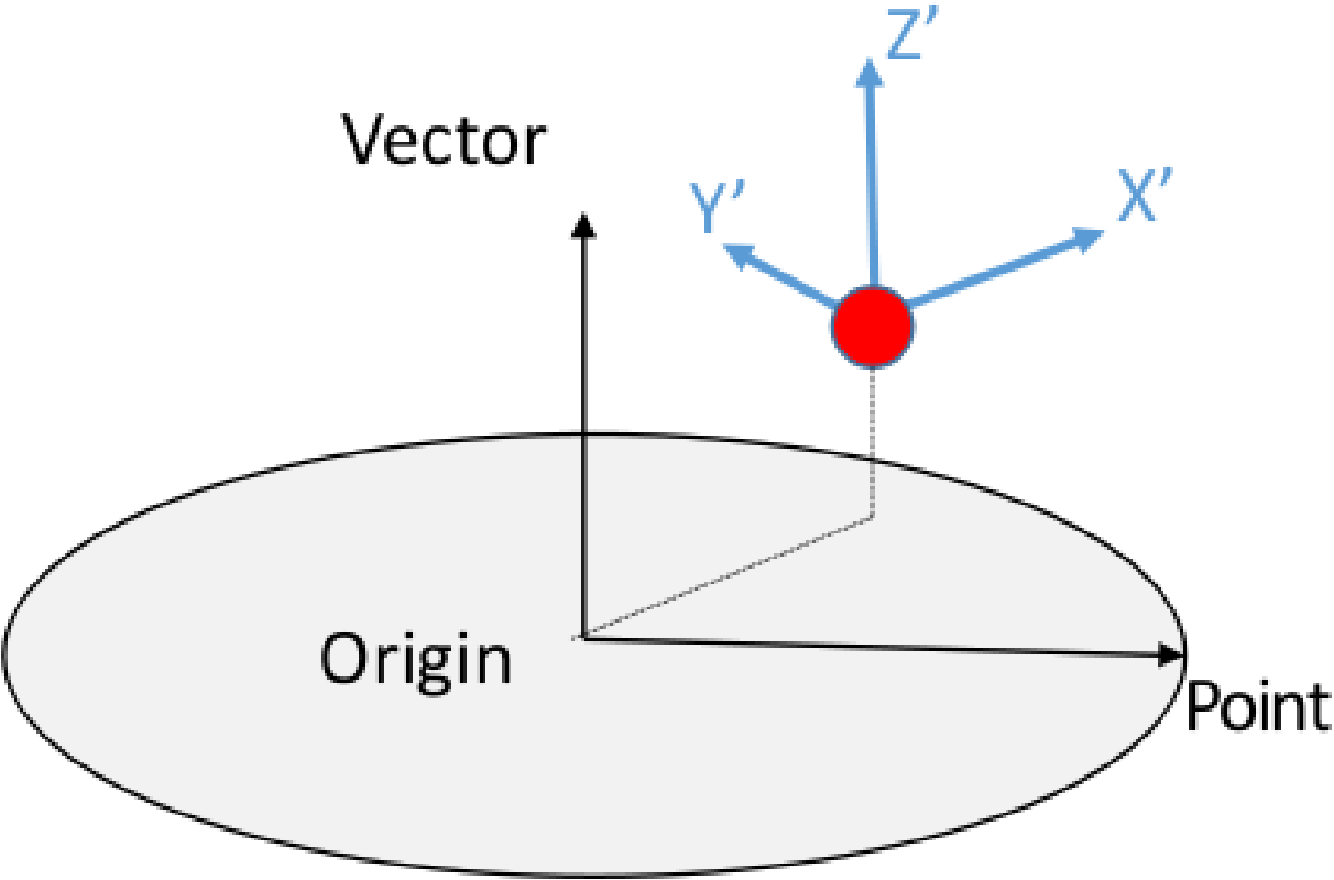
Fig. 9.1 Default cylindrical transformation.
The nodal fields coordinates and model_coordinates are treated specially. These positional vectors are transformed to new positions in the target coordinate system. This special position transformation only applies to these two specific nodal field names. For cylindrical coordinate system the coordinate vectors are transformed into R \(\Theta\) Z coordinates where \(\Theta\) is in radians as shown in Figure Fig. 9.2.
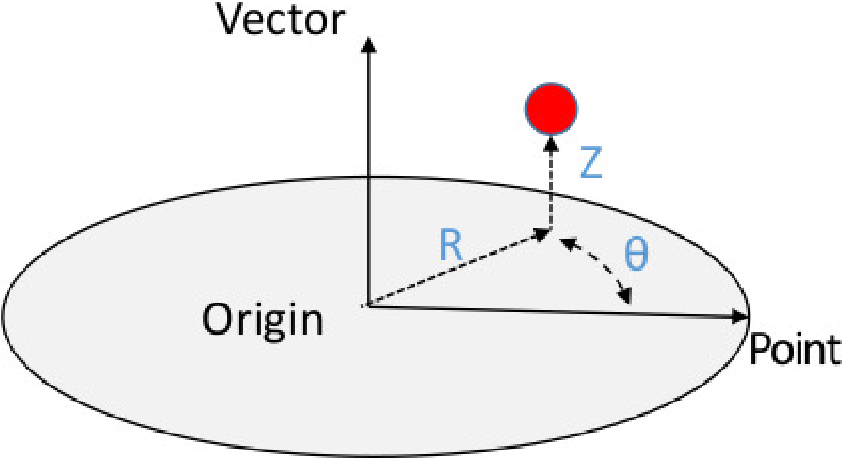
Fig. 9.2 Cylindrical system transformation of coordinates.
Warning
This command cannot be used to transform shell element tensors which are not computed in the global coordinate system. Output of shell stress and strain components in a user-defined, local co-rotational coordinate system are obtained with the element variables transform_shell_stress and transform_shell_strain as described in Section 9.3.1.
Warning
If all elements used to track and update the coordinate system in this command are killed via element death, the coordinate system will not update anymore, and will be zeroed-out. In this setting, all transformed output using this coordinate system will also be zeroed-out for the remainder of the simulation. See Section 2.1.10 for details.
9.4.7. Data Filtering Commands
BEGIN FILTER <string>filter_name
  ACOEFF = <real_list>a_coeff
  BCOEFF = <real_list>b_coeff
  INTERPOLATION TIME STEP = <real>ts
END [FILTER]

BEGIN USER OUTPUT
  FILTER <string>new_var FROM {GLOBAL|NODAL|ELEMENT|FACE}
    <string>source_var USING <string>filter_name
END
The user output FILTER command creates a new variable new_var by performing an on-the-fly frequency filter of the named element, nodal or face variable source_var. The BEGIN FILTER command block defines a filter with the name filter_name. The filter defined by the begin filter command block is then referenced by the USER OUTPUT filter command.
In the BEGIN FILTER command block the A and B filtering coefficients are defined with the ACOEFF and BCOEFF command lines. The filter must define at least one A and one B coefficient, there is no maximum number coefficients and the length of A and B do not need to match.
Filter operations assume that the data given at a constant time step. The explicit dynamics time step will tend to vary during the analysis. The INTERPOLATION TIME STEP command is used to linearly interpolate the data being produced at a non-constant time step down to some specified constant time step. The interpolation time step must be larger than zero and ideally should be specified to be smaller than the smallest time step with which the computations will iterate.
One way to obtain the filtering coefficients is with MATLAB. The following is an example of defining a third order Butterworth filter with a pass frequency of 100Hz at data interpolated to a time step of \(1.0e-5\) seconds. The filter is then used to filter acceleration histories of the nodes to 100Hz. The MATLAB code below will give the desired filtering coefficients. The full 16-digit precision of the coefficients returned by MATLAB should be used. If truncated precision numbers are used, the filters can potentially be unstable.
clear;
format long e;
passFrequency = 100;
interp_ts = 1.0e-5;
butterCoeff = 2.0*interp_ts*passFrequency;
[bcoeff,acoeff] = butter(3,butterCoeff);
acoeff
bcoeff
The computed filtering coefficients can be used in a USER OUTPUT block as show below. If the analysis time step always remains above \(1.0e-5\) the filter will be valid. If the analysis time step drops below \(1.0e-5\) there could be aliasing issues, and a smaller interpolation time step should be specified.
BEGIN FILTER filt_100Hz
  ACOEFF = 1.000000000000000e+00 -2.987433650055722e+00 \$
           2.974946132665442e+00 -9.875122361107358e-01
  BCOEFF = 3.081237301416628e-08  9.243711904249885e-08 \$
           9.243711904249885e-08  3.081237301416628e-08
  INTERPOLATION TIME STEP = 1.0e-5
END
BEGIN USER OUTPUT
  FILTER ax100Hz FROM NODAL acceleration(x) USING filt_100Hz
  FILTER ay100Hz FROM NODAL acceleration(y) USING filt_100Hz
  FILTER az100Hz FROM NODAL acceleration(z) USING filt_100Hz
END
9.4.8. Nonlocal Averaging
BEGIN NONLOCAL AVERAGE <string>name
  SOURCE VARIABLE = NODAL|ELEMENT <string>variable_name
  TARGET VARIABLE = NODAL|ELEMENT|GLOBAL <string>variable_name
  RADIUS = <real>radius_value
  POINT = <real>x <real>y <real>z
  #options only for nodal nonlocal averaging
  NUMBER OF RINGS = <int>num_rings
  DISTANCE WEIGHTING FUNCTION = <string>function_name
  DISTANCE ALGORITHM = EUCLIDEAN_DISTANCE |
                       GRAPH_DISTANCE | EUCLIDEAN_GRAPH
  WEIGHTING VARIABLE = <string>nodal_weighting_variable_name
  PRINT DEBUG INFORMATION FOR NODE = <int>node_id
  #option only for element nonlocal averaging
  SAMPLE POINTS IN SPHERE AT RADIAL INCREMENT
          <real>increment AND ANGLE <real>angle
  OUTPUT IN LOCAL COORDINATE SYSTEM <string>coord_sys_name
END
The NONLOCAL AVERAGE computes weighted averages over all nodes or elements inside spherical domains with size defined by the RADIUS or a set number of mesh layers out from the source node defined by the NUMBER OF RINGS. The search for points inside each domain is performed once during initialization, so the domains are defined in initial model coordinates. A GLOBAL result_var_name will perform nonlocal averaging over a single domain and requires a POINT to define the center of this domain. A NODAL or ELEMENT result_var_name will perform nonlocal averaging at every included mesh entity by creating a domain with the specified radius at every mesh entity. A NODAL result_var_name requires a NODAL source_var_name and an ELEMENT result_var_name requires an ELEMENT source_var_name.
By default, a nonlocal average over a nodal source variable is mass-weighted and a nonlocal average over an element source variable is volume-weighted. Additionally, a DISTANCE WEIGHTING FUNCTION can be used to specify the weighting used for nodal variables. The formula for the distance weighting is
where \(x(n)\) is the source value at node \(n\), \(d(n)\) is the distance node \(n\) is away from the target node, and \(w(d(n))\) is the weight function evaluated at \(d(n)\). An example input deck setup that uses the weighting function is shown below.
BEGIN FUNCTION include_everything_but_me
  TYPE IS PIECEWISE LINEAR
  BEGIN VALUES
    0.0      0.0
    1.0E-6   1.0
    3.0      1.0
  END VALUES
END

BEGIN NONLOCAL AVERAGE avg1
  SOURCE VARIABLE = NODAL contact_status
  TARGET VARIABLE = NODAL averaged_contact_status
  RADIUS = 2.0
  DISTANCE WEIGHTING FUNCTION = include_everything_but_me
END
A WEIGHTING VARIABLE may also be specified and used in combination with the DISTANCE WEIGHTING FUNCTION. The weighting variable may be any nodal variable used in Sierra/SM .
There are currently three different distance algorithms that can be used for nonlocal averaging: EUCLIDEAN_DISTANCE, GRAPH_DISTANCE, and EUCLIDEAN_GRAPH.
The EUCLIDEAN_DISTANCE option simply computes the distance between the source and target entity. No considerations are taken with respect to the mesh graph in this method.
The GRAPH_DISTANCE option starts at the source entity and walks the edges of the mesh to find connected target entities. As the mesh is walked, the graph distance is computed. If the graph distance from the source entity to the target entity is less than the given radius, the target entity is included in the kernel.
The EUCLIDEAN_GRAPH option walks the mesh and only finds entities within the sphere that are connected to the source entity. This algorithm first does a EUCLIDEAN search to get a set of nodes within the sphere. Then, the mesh is walked from the source node, and grabs all nodes connected to the source node, and recursively continues. Nodes outside of the euclidean set are not included and stop the recursion.
For nodal nonlocal averaging, debugging information may be printed to the logfile with the PRINT DEBUG INFORMATION FOR NODE command. Debugging information will be printed for all nodes specified in the line command.
For element nonlocal averaging, lower order integration may be specified via the SAMPLE POINTS IN SPHERE AT RADIAL INCREMENT <real>increment AND ANGLE <real>angle command. Instead of including every element that lies within the domain of the sphere, the elements are only included if a point specified by the above line command lies within the element. This line command will significantly improve performance of the algorithm, but in general, may be less accurate than including every element in the domain.
When creating a global target variable in nonlocal averaging, the user has the option to output the global variable in a local coordinate system. This can be accomplished via the OUTPUT IN LOCAL COORDINATE SYSTEM line command. When specifying this command, the user can optionally specify the name of the local coordinate system to move. If it is desired to create and specify your own local coordinate system, please refer to Section 2.1.10 for the syntax to create your moving coordinate system. If no coordinate system is specified, the coordinate system will be created automatically and given the name specified in the BEGIN NONLOCAL AVERAGE command block. The coordinate system will be initially aligned with the global XYZ coordinate system, and it will move with the block, surface, or nodeset specified in the BEGIN USER OUTPUT command block. When automatically computing the coordinate system, the coordinate system vector visualization is set to ON.
The OUTPUT IN LOCAL COORDINATE SYSTEM <string>coord_sys command will cause the output to be with respect to a local coordinate system previously defined within Sierra scope. If no local coordinate system name is given, a local coordinate system centered about the nonlocal domain will be constructed with the name <nonlocal_domain_name>_COORDINATE_SYSTEM. This feature is only supported for GLOBAL target variables.
9.4.9. Compute at Every Step Command
COMPUTE AT EVERY STEP
If this command line appears in the USER OUTPUT command block, a user-defined variable in the command block will be written at every time step. Section 10.2.4 discusses user-defined variables.
!explicit!
In explicit dynamics analyses, user-defined variables can be used as criteria for element death. In this case, the COMPUTE AT EVERY STEP command must be used to force those variables to be computed at every time step. See Section 6.5 for more information on element death.
9.4.10. Additional Commands
Active and Inactive Periods Commands
ACTIVE PERIODS = <string list>period_names
INACTIVE PERIODS = <string list>period_names
The ACTIVE PERIODS and INACTIVE PERIODS command lines determine when the USER OUTPUT command block is either active or inactive. See Section 2.6 for more information about this optional command line.
Compute at Output Steps Commands
COMPUTE AT {HEARTBEAT|HISTORY|RESULTS} OUTPUT STEPS \#
      DATABASE NAME <string>database_name
This command line specifies to compute the current user output block at only heartbeat, history, or results output steps associated with a particular database. For instance, if a particular USER OUTPUT command block is computationally intensive, but the results of the user output computation are only needed at relatively infrequent results output intervals, specifying COMPUTE AT RESULTS OUTPUT STEPS would exclude the user output block from being computed at history and heartbeat output steps and could result in a significant simulation runtime savings.
If this command line is not specified anywhere in a USER OUTPUT command block, the block will be computed at all output steps. It is admissible to specify multiple COMPUTE AT OUTPUT STEPS command lines per USER OUTPUT command block, for instance, if it is desired to compute at both history and heartbeat output steps.
9.4.11. Sensors
BEGIN SENSOR <string>sensor_name
  #
  # mesh-entity set commands
  NODE SET|NODESET = <string list>nodelist_names
  SURFACE = <string list>surface_names
  BLOCK = <string list>block_names
  ASSEMBLY = <string list>assembly_names
  INCLUDE ALL BLOCKS
  # source variable command
  SOURCE VARIABLE = ELEMENT|NODAL <string> field_name
  #coordinate system commands
  ALIGN COORDINATE SYSTEM WITH GLOBAL_XYZ
  ALIGN COORDINATE SYSTEM WITH ENTITY <string> block_name|
    surface_name|nodeset_name
  COORDINATE SYSTEM = <string> user_coordinate_system_name
  #compute commands
  COMPUTE OVER NONLOCAL SPHERE DOMAIN DEFINED BY
    RADIUS <real>radius AND POINT <real>x <real>y <real>z
  OPERATION = AVG|MAX|MIN
END [SENSOR]
The SENSOR command block enables the user to generate output on a mesh entity or nonlocal domain in a specific coordinate frame. More than one sensor can be specified. Sensor outputs can be used to compare against accelerometer or strain gauge experimental data. The command block appears inside the region scope. Specifying a sensor adds a global variable with the name sensor_name.
The SENSOR command block contains four groups of commands–mesh-entity set, source variable, coordinate system, and compute.
9.4.11.1. Mesh-Entity Set Commands
The mesh-entity set commands portion of the SENSOR command block specifies the nodes, element faces, elements, or assemblies associated with the sensor. This portion of the command block can include some combination of the following command lines:
NODE SET|NODESET = <string list>nodelist_names
SURFACE = <string list>surface_names
BLOCK = <string list>block_names
ASSEMBLY = <string list>assembly_names
INCLUDE ALL BLOCKS
These command lines, taken collectively, constitute a set of Boolean operators for constructing a set of nodes, element faces, or elements. There must be exactly one NODE SET|NODESET, SURFACE, BLOCK, INCLUDE ALL BLOCKS, or ASSEMBLY command line in the command block. Assemblies may contain blocks, surfaces, nodesets, or assemblies of these.
All nodes in the entity will be grabbed. A local coordinate system is created and aligned with the principal axis computed from the entity.
9.4.11.2. Source Variable Command
SOURCE VARIABLE = ELEMENT|NODAL <string> field_name
The SOURCE VARIABLE command line is used to specify the element or nodal variable that is to be computed in the local coordinate system. The source variable is required to be specified. The source variable can be a scalar, vector, or tensor field.
9.4.11.3. Coordinate System Commands
ALIGN COORDINATE SYSTEM WITH GLOBAL_XYZ
ALIGN COORDINATE SYSTEM WITH ENTITY <string> block_name|
  surface_name|nodeset_name
COORDINATE SYSTEM = <string> user_coordinate_system_name
The optional coordinate system commands are used to specify the coordinate system with which the entity will be aligned.
The ALIGN COORDINATE SYSTEM WITH GLOBAL_XYZ command line aligns the coordinate system with the global coordinate system.
The ALIGN COORDINATE SYSTEM WITH ENTITY command line aligns the coordinate system with the entity specified.
The COORDINATE SYSTEM command line allows the specification of a user-defined coordinate system. The user-defined coordinate system must be specified as moving. See Section 2.1.10.
The ALIGN COORDINATE SYSTEM WITH ENTITY and COORDINATE SYSTEM command lines may not be specified simultaneously, as this would be a conflicting specification.
9.4.11.4. Compute Commands
COMPUTE OVER NONLOCAL SPHERE DOMAIN DEFINED BY
  RADIUS <real>radius AND POINT <real>x <real>y <real>z
OPERATION = AVG|MAX|MIN|SUM
The optional COMPUTE OVER NONLOCAL SPHERE DOMAIN DEFINED BY command line is used to specify the nonlocal spherical domain over which the source variable is to be computed in the local coordinate system.
The optional OPERATION command line is used to specify the operation when computing the source variable in the local coordinate system. Specifying AVG computes the average of the variable, MAX computes the maximum, and MIN computes the minimum. Each operation is performed component-by-component on vector and tensor fields. Additionally, the MAX and MIN commands are performed on fields with respect to the global reference frame.
The average is the default operation.
For a more thorough walkthrough of the various sensor options, please see Section 9.5.
9.4.12. Chaining together multiple user output operations
When having user output operations where the result of one depends on the result of the other, it is recommended to create user variables with the same name.
For example, the global variable resulting from taking the average of a nodal variable is subsequently used in a filter command. It would be advisable to create a global user variable of the same name, so in this case:
begin user variable Ax
  type = global real length = 1
  global operator = max
  initial value = 0
end

begin user output
  block = block_1
  compute global Ax as average of nodal acceleration
  filter accel_filter from global Ax using filter_frequencies
end
Refer to Section 10.2.4 for the syntax for user variables.