9.5. Sensor Examples

The following examples show various ways in which sensors can be set-up and used.

First, consider the following straight beam:

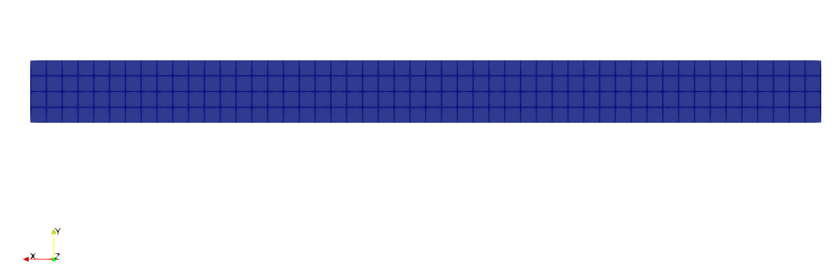
../../_images/straightBeam.png — Fig. 9.3 Straight beam example

For this problem, the beam is subjected first to a pure rotation followed by a rotation and a translation.

../../_images/rotatingBar.gif — Fig. 9.4 Straight beam example

After meeting with your customer, it has been communicated to you that there is an accelerometer at the tail end of the beam. The accelerometer data is one of the main QOIs for this problem, and your customer would like to model its output. To model this accelerometer in Sierra/SM, you have various different options, each with different pros and cons.

9.5.1. Initial Alignment with the Global XYZ Axes

The first method of creating a sensor is by specifying an entity for which to average the accelerations over (surface_10 in this case), and how to initially align the local coordinate system (GLOBAL_XYZ in this case). As you can see, the r, s, and t vectors are initially aligned with the global x, y, and z directions, but these r, s and t vectors move as the average motion of all of the nodes in surface_10.

BEGIN SENSOR accelerometer_tail
  SURFACE = SURFACE_10
  SOURCE VARIABLE = NODAL ACCELERATION
  ALIGN COORDINATE SYSTEM WITH GLOBAL_XYZ
END

../../_images/coordSysDirs.gif — Fig. 9.6 r, s, and t vectors of the local coordinate system. In this problem, the rdir is green, the sdir is yellow, and the tdir is red.

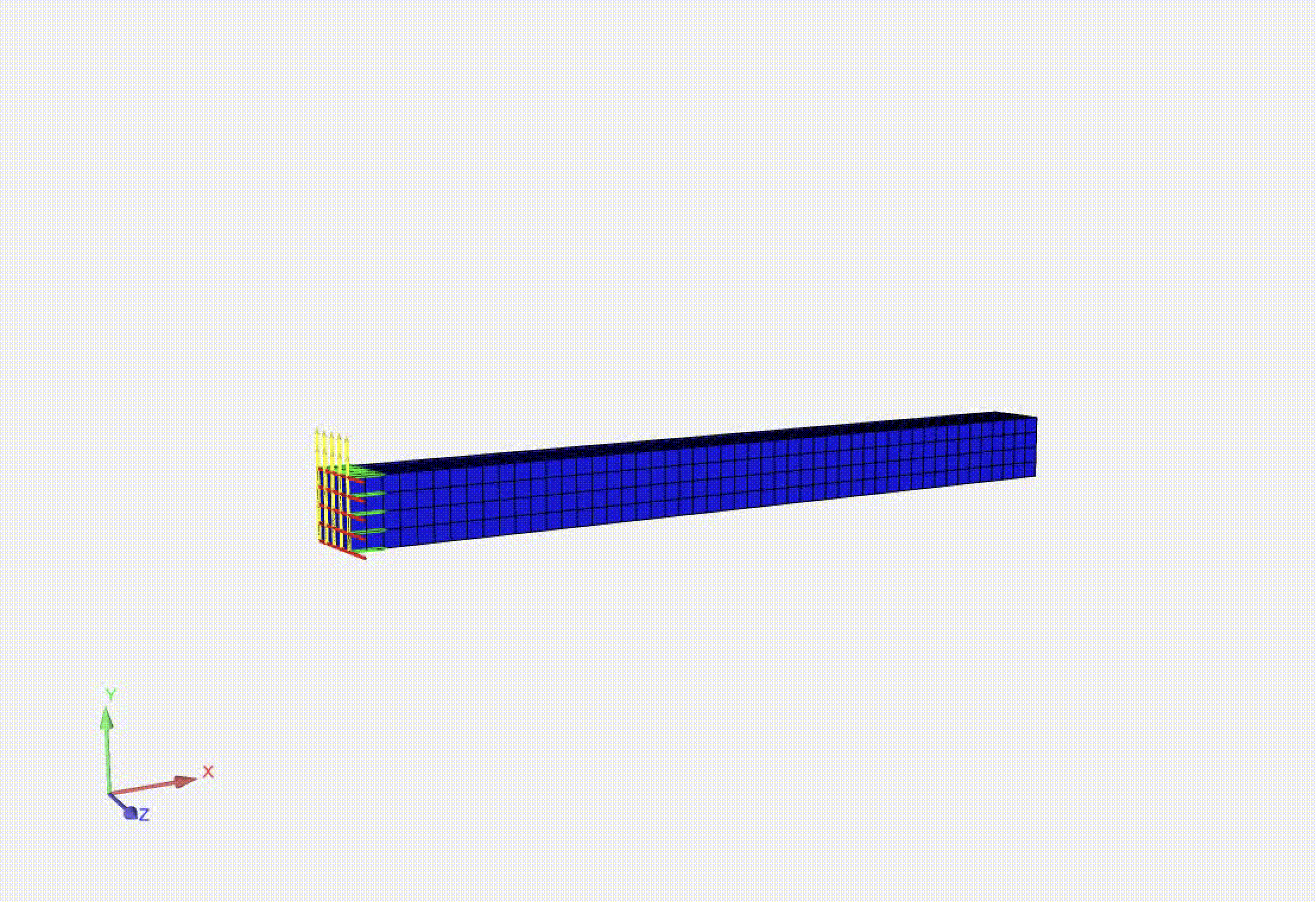
../../_images/coordSysDirs.png — Fig. 9.7 r, s, and t vectors of the local coordinate system. In this problem, the rdir is green, the sdir is yellow, and the tdir is red.

Note that the r, s and t vectors can be output and visualized on your model by adding the following to your results output block:

BEGIN RESULTS OUTPUT OUT1
   ...
   NODAL VARIABLES = accelerometer_tail_1_rdir
   NODAL VARIABLES = accelerometer_tail_1_sdir
   NODAL VARIABLES = accelerometer_tail_1_tdir

Where accelerometer_tail_1 is the name of your sensor. While this is probably the easiest option to implement, note that the sensors in the experimental setup must be aligned with the global XYZ axes.

9.5.2. Initial Alignment Specified Via Three Nodesets

If your accelerometer is not aligned with the global XYZ axes, there are other ways to specify the initial orientation of the coordinate system. One such option is to specify the initial coordinate system alignment within the rectangular coordinate system.

BEGIN RECTANGULAR COORDINATE SYSTEM LOCAL_CS_1
   ORIGIN NODESET = NODELIST_101
   Z POINT NODESET = NODELIST_102
   XZ POINT NODESET = NODELIST_103
END

In this example, the nodesets are oriented as such:

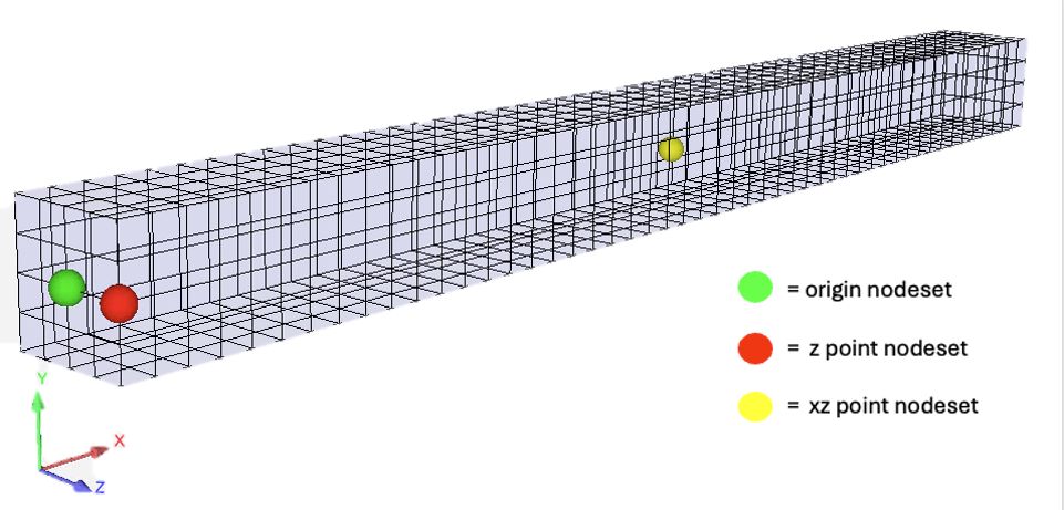
../../_images/beamNodesetPositions.png — Fig. 9.8 Nodesets defined on the bar

Note that each nodeset must contain one and only one node. The coordinate system is then used directly in the sensor as such:

BEGIN SENSOR accelerometer_ns_tail
  SURFACE = SURFACE_10
  SOURCE VARIABLE = NODAL ACCELERATION
  COORDINATE SYSTEM = LOCAL_CS_1
END

In this case, the average acceleration is computed over all of the nodes specified in surface_10, and the average quantity is rotated via the rotation computed by the three nodes in each nodeset (NODELIST_101, NODELIST_102, and NODELIST_103). Because of this, this option will be slightly more performant than the other options.

Warning

Note that if any of the nodes in the three nodesets are killed, a rotation can no longer be computed and the output of the sensor will be invalid.

9.5.3. Initial Alignment Specified Via Three Nodesets But Rotation Computed Separately

If you like the option of specifying the initial configuration via nodesets, but you would like to ensure your sensor will continue to compute correctly with element death, a TRACKING ENTITY can be specified to compute the rotations.

BEGIN RECTANGULAR COORDINATE SYSTEM LOCAL_CS_1
   ORIGIN NODESET = NODELIST_101
   Z POINT NODESET = NODELIST_102
   XZ POINT NODESET = NODELIST_103
   SYSTEM = MOVING
   TRACKING ENTITY = SURFACE_10
END

This coordinate system is then used in the sensor in the same way as the prior example:

BEGIN SENSOR accelerometer_ns_track_tail
  SURFACE = SURFACE_10
  SOURCE VARIABLE = NODAL ACCELERATION
  COORDINATE SYSTEM = LOCAL_CS_1
END

9.5.4. Sensor Computed Across a Nonlocal Spherical Domain

Another convenient option for creating sensors is to specify the calculation domain via a nonlocal spherical domain. This comes in hands when it is inconvenient to mesh an accelerometer entity (such as a block or a sideset) or when the accelerometer location may change. The syntax to create a sensor for a nonlocal sphere is as follows:

BEGIN SENSOR accelerometer_nonlocal_tail
  BLOCK = BLOCK_10
  SOURCE VARIABLE = NODAL ACCELERATION
  COMPUTE OVER NONLOCAL SPHERE DOMAIN DEFINED BY RADIUS 0.05 AND POINT -2.5 0.0 0.0
  ALIGN COORDINATE SYSTEM WITH GLOBAL_XYZ
END

By doing this, we are able to specify the entire block for the sensor, but the nonlocal sphere domain limits the nodes we are averaging to just those on the tail of the bar. The accelerations are averaged over just the nodes that fall within the sphere, and the QOI is rotated using the rotation matrix computed over all of the nodes in the main entity specified (BLOCK_10 in this case).

The results of each of the methods are plotted below. Note that because the rotations are computed with the three individual nodes in sensor accelerometer_ns_tail, we get a nontrivial acceleration in the z direction. However, for all of the other sensors, the acceleration in the z direction is very close to zero.

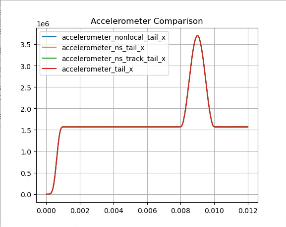
../../_images/accelsX.png — Fig. 9.9 Accelerations in the local X direction

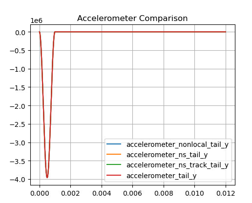
../../_images/accelsY.png — Fig. 9.10 Accelerations in the local Y direction

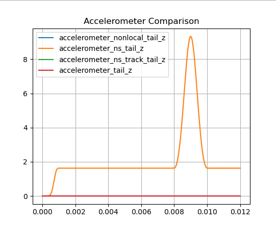
../../_images/accelsZ.png — Fig. 9.11 Accelerations in the local Z direction