8.9. Contact Algorithm Options
8.9.1. Contact Library
SEARCH = DASH(DASH)
Dash is the only supported search and enforcement algorithm for both explicit dynamics or implicit contact. ACME, the other previously available search algorithm, has been deprecated. Any usage of ACME search should be discontinued and any resulting issues should be reported to sierra-help.
8.9.1.1. The Dash algorithm
Dash offers a facet-based enforcement algorithm. By default, Dash enforces face-face constraints. Dash also offers a node-face based enforcement algorithm.
Dash is designed to work correctly for a wide variety of problems with minimal user intervention. It is generally recommended that Dash be used with a minimal set of inputs, for example skin all blocks, self contact = on, and/or general contact = on, and definition of the needed interaction friction models. Dash ignores tangential tolerances for face/face constraints. For more details, see discussion in Section 8.9.1.2.
For explicit contact, Dash uses an iterative augmented Lagrange enforcement scheme, applying equal and opposite forces.
For implicit contact, the Dash contact search can be used with either kinematic or augmented Lagrange enforcement. When Dash is used with the implicit kinematic enforcement algorithm, only node-face interactions are enforced, and the default behavior is changed from face-face to node-face.
Dash can only represent shells via lofted geometry and has no option to treat shells as if they have no thickness for contact. A zero-thickness contact surface on shells can be achieved by using a sideset surface definition, however this contact surface will be one-sided. If the sideset approach is taken, then the surface normal will define the contact side. Dash adds the edge faces to lofted shells, allowing edge and edge to face contact to function correctly on shell elements. Dash also handles beam on beam contact via lofted geometry. Beam objects are turned into representative hexagonal prisms that have roughly the same cross sectional area that the beam elements have. Beam contact is functional for edge-on or end-on cases.
8.9.1.2. Dash Usage Guidelines
Dash is robust on problems with element death.
When performing contact involving shells, beams, and particles, Dash turns the elements into lofted volumes.
Prefer using block skinning with Dash, and avoid defining contact surfaces based on side sets. Dash uses ray tracing algorithms to determine if certain contact points are inside or outside of bodies. If the surfaces used for contact with Dash do not define fully enclosed bodies, it is difficult for the algorithm to determine whether a point is inside or outside a body.
8.9.2. Dash Specific Options
BEGIN DASH OPTIONS
  INTERACTION DEFINITION SCHEME = {EXPLICIT|AUTOMATIC} (AUTOMATIC)
  SEARCH LENGTH SCALING = <real>scale(0.15)
  TIED SEARCH LENGTH SCALING = <real>scale(0.25)
  SUBDIVISION LEVEL = <int>sublevel(0)
  QUAD PROJECTION TYPE =
    {TRIANGULAR_FACETS|QUAD}(TRIANGULAR_FACETS)
  HIDDEN SELF CONTACT POSSIBLE = FALSE|TRUE (TRUE)
  MAX CONTACT SUB STEPS = <int>maxSteps(100)
  NODE NORMAL SMOOTHING = AREA_WEIGHTED|ANGLE_WEIGHTED (ANGLE_WEIGHTED)
  SEPARATE DISCONNECTED MESH COMPONENTS =
    {TRUE|FALSE|ANGLE_BASED}(FALSE) <real>threshold(0.707)
END
The DASH OPTIONS command block contains a few options unique to Dash. Generally Dash is designed to run accurately with as few user specified parameters as possible, however, some extra options are available. Note, the options in this block should generally be used only by experienced analysts for specific purposes.
The INTERACTION DEFINITION SCHEME command controls how contact interactions are defined. By default, most Dash interactions are one sided and the full volume of overlap is removed. By default, Dash automatically picks an optimal enforcement order for each interaction pair based on face size. However, the ability exists to explicitly use the interactions defined in the input deck by supplying the EXPLICIT option to this command. This may allow better control of interaction setup in some circumstances or can be used to force Dash to use a symmetric interaction when it would by default use a one sided interaction. For example, when two surfaces s1 and s2 appear in an interaction definition using the SURFACES line command, the EXPLICIT option for INTERACTION DEFINITION SCHEME will automatically establish a symmetric interaction. In such an interaction, s1 will be the SIDE B (with s2 as the SIDE A) as well as the SIDE A (with s2 as the SIDE B).
The SEARCH LENGTH SCALING command is used to control how Dash computes automatic contact tolerances. The automated search length used by contact at each face is the characteristic size of the face times this value. Note that the default value of this command should be used in almost all circumstances. One use of this command is to zero the automatic tolerances to force the contact algorithm to use the user provided search tolerances (normally contact uses the larger of the user provided or the default search tolerance). In some cases such as high velocity contact where objects move further than the default search length over a single step use of a larger factor can be helpful. Increasing the SEARCH LENGTH SCALING parameter may also be used to help resolve interpenetration issues in implicit contact that arise from large motion over a single time step. In such cases, values as large a 1.0 may be necessary. Note though that use of a scaling factor larger than approximately 0.50 can cause instability in the contact solution, especially for thin-walled structures, and should be used with caution in such cases.
Tied interactions used the length scaling given by TIED SEARCH LENGTH SCALING, by default tied interactions use a somewhat larger search length. If a tied interaction is initially further than the characteristic face size times the search length scaling tied contact will not be found. A larger or smaller value for this scaling number can be provided. However, values larger than 0.50 should be avoided as they can result in instability.
The SUBDIVISION LEVEL command provides a means to force a triangular face to be subdivided. Each quadrilateral face is originally split into four triangular faces. A subdivision level splits each tri-face edge into sublevel+1 segments. An increased subdivision level give a more accurate solution because the overlap volume is more accurately calculated. This increased accuracy, however, comes with a significantly increased computational cost.
The QUAD PROJECTION TYPE command provides a means to select the projection scheme of contact interactions to potentially warped quad surfaces. The default TRIANGULAR_FACETS option computes the projection point by dividing each quad into four flat triangles. The QUAD option computes the true position of the projection point on the warped quad. The TRIANGULAR_FACETS is faster to compute and is more robust in loading where deformations and potential warping is large. The QUAD option is somewhat more expensive to compute but can give a more consistent numerical result in an analysis where deformation is small.
The HIDDEN SELF CONTACT POSSIBLE command is used to control how Dash automatically sets up interactions. Self contact interactions use special more expensive contact logic. This more complex logic is needed to resolve constraint chaining issues that can happen in self contact. If two surfaces share (say contiguous blocks) and those two surfaces contact then by default the contact logic is applied as well as the same constraint chaining issues arise. The HIDDEN SELF CONTACT POSSIBLE command can be used to turn off this more expensive self contact logic. This can sometimes improve performance but may introduce instabilities in the contact solution.
In high velocity contact situations explicit contact enforcement may subdivide the time step to help accurately capture interactions. The MAX CONTACT SUB STEPS can be used to set the maximum number of sub steps taken over a step. In practice the only use of this command would be to drop number of sub steps taken to one in a problem that is encountering some issue with the sub stepping computations.
8.9.2.1. Node Normal Smoothing
BEGIN DASH OPTIONS
  NODE NORMAL SMOOTHING = AREA_WEIGHTED|ANGLE_WEIGHTED(ANGLE_WEIGHTED)
END
The NODE NORMAL SMOOTHING affects how the nodal normals are computed for Dash node/face contact. The node normal is used to determine which face a given node will contact. In cases were multiple faces are potential contact candidates the node will contact the face with the face normal that most opposed the node normal.
There are two options for normal smoothing. The default ANGLE_WEIGHTED option computes the nodal normal as the sector angle weighted normals of attached faces. Consider the example shown in Fig. 8.18 two faces come together at right angles. The sector angle (the angle at the face corner that attaches to the node) of both faces is 90 degrees. Thus the two faces contribute equally to the node normal which is at 45 degrees. The AREA_WEIGHTED option computes the nodal normal as the face angle weighted normals of attached faces. In Fig. 8.18 the top face has more area than the side face. This pulls the node normal more in the direction of the top face.
The ANGLE_WEIGHTED is generally more accurate and has several beneficial property. With the angle weighted normal the node normal at edges and corners is not dependent on the specific mesh or element shapes. This is a very useful property for convergence studies. Additional for any convex geometry the angle weighted normal is guaranteed to be at least partially aligned with all attached face normals. This can make finding corner node/face interactions more robust. The primary advantage of the AREA_WEIGHTED option is speed. Use of the AREA_WEIGHTED option can improve runtime by up to 20% in some cases. Additionally the AREA_WEIGHTED option was the Sierra/SM default behavior before version 4.46 and is maintained for backward compatibility.
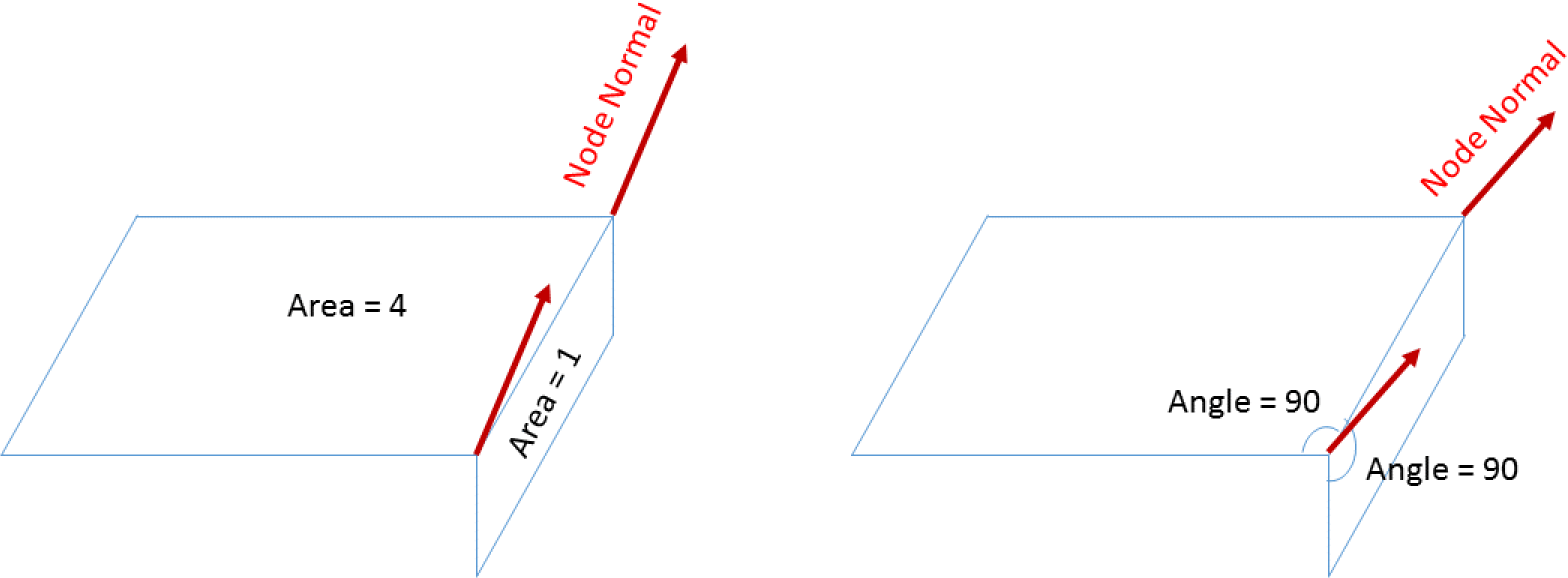
Fig. 8.18 Node normal computation options.
8.9.2.2. Separate Disconnected Mesh Components
BEGIN DASH OPTIONS
  SEPARATE DISCONNECTED MESH COMPONENTS =
    {TRUE|FALSE|ANGLE_BASED}(FALSE) <real>threshold(0.707)
END
The SEPARATE DISCONNECTED MESH COMPONENTS command allows for partitioning of contact surfaces automatically. TRUE partitions contact surfaces according to mesh connectivity. ANGLE_BASED will also partition contact surfaces according to mesh connectivity and additionally group adjacent faces that share a similar normal. threshold allows for specification of how similar normals need to be in order to group the faces, the threshold value represents the cosine of the angle between the normals. Adjacent faces with cosine angles greater than the threshold are grouped together. Partitioned surfaces inherit settings from the original contact surface: friction model, self contact, etc. Visualization of the partitioned surfaces can be viewed using the face variable surface_partition_id.
Warning
Currently, this option can not be used with the Dash visualization options or when outputting certain contact variables. The simulation will run, but a warning will print to the log file.
![]()
8.9.3. Enforcement
ENFORCEMENT = <string>AL|KINEMATIC(AL)
CONTACT RESIDUAL NORM SCALE FACTOR = <real>scale
The ENFORCEMENT command line controls whether kinematic or Augmented Lagrange (AL) enforcement will be used in the current CONTACT DEFINITION block.
The AL option enforces contact using an Augmented Lagrange algorithm. This option can be used only in conjunction with the Dash search, which is enabled using the SEARCH = DASH command (See Section 8.9.2), and is the default option when using the Dash search. The FRICTION MODEL commands are necessary with this command and varying contact models can be enforced within the same CONTACT DEFINITION block.
If kinematic enforcement is enabled (by using the KINEMATIC option), the enforcement algorithm and the friction model are linked, and only one friction model can be used per CONTACT DEFINITION block. If a combination of tied, frictionless, and frictional contact is to be enforced, multiple CONTACT DEFINITION blocks must be included in the input file.
The CONTACT RESIDUAL NORM SCALE FACTOR Applies scale factor to contact residual norm of the contact definition in which this command is embedded. This allows a specific contact definition to contribute with different weight factor to the total contact residual norm. For example, one may want the contact residual from ARS to be the only contribution to the contact residual norm. This can be achieved by suppressing all other contributions using a scale factor of 0. The default value is unity.
8.9.4. Remove Initial Overlap
INITIAL OVERLAP REMOVAL = <string>ON|OFF(OFF)

BEGIN REMOVE INITIAL OVERLAP
  OVERLAP NORMAL TOLERANCE = <real>over_norm_tol
  OVERLAP TANGENTIAL TOLERANCE = <real>over_tang_tol
  OVERLAP ITERATIONS = <integer>iterations(100)
  DEBUG ITERATION PLOT = <string>ON|OFF(OFF)
  IGNORE KINEMATIC CONSTRAINTS = <string>ON|OFF(OFF)
  PRINT ALL DEBUGGING DATA = <string>ON|OFF(OFF)
  REMOVE OVERLAP AT START OF TIME PERIODS = <string list>periods
  SETTINGS = OLD|IMPROVED(OLD)
END REMOVE INITIAL OVERLAP

OVERLAP REMOVAL ONLY = OFF|ON(OFF)
Meshes supplied for finite element analyses often have some level of initial mesh overlap, where finite element nodes reside inside the volume of nearby elements. In particular, this will happen when meshes meet at non-contiguous curved boundaries.
In explicit analyses the contact algorithm will attempt to push the overlapped constraints to zero gap. If a mesh has initial overlap contact will attempt to push out that overlap over the first explicit time step. As the explicit time step is often small, this may result in an extremely large force, velocity, and energy input into the initial mesh. Additionally, these initial forces are nonphysical and may produce erroneous stress waves. Initial overlap removal is a mechanism for modifying the initial mesh to eliminate any initial overlap of contact surfaces. This is done before taking the first explicit dynamics time step to avoid the aforementioned issues. The overlap removal algorithm is by default turned off, but can be turned on by including the INITIAL OVERLAP REMOVAL = ON command line or use of the BEGIN REMOVE INITIAL OVERLAP block. The REMOVE INITIAL OVERLAP command block can also be used to modify the default overlap removal settings described later in this section.
For an example of overlap removal, see Fig. 8.19.
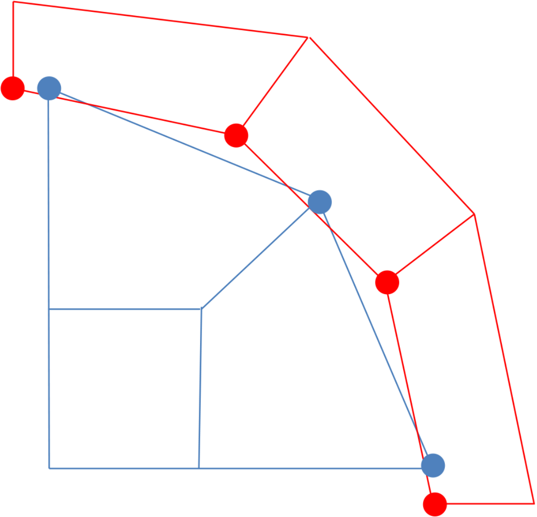 (a) Initial geometry.
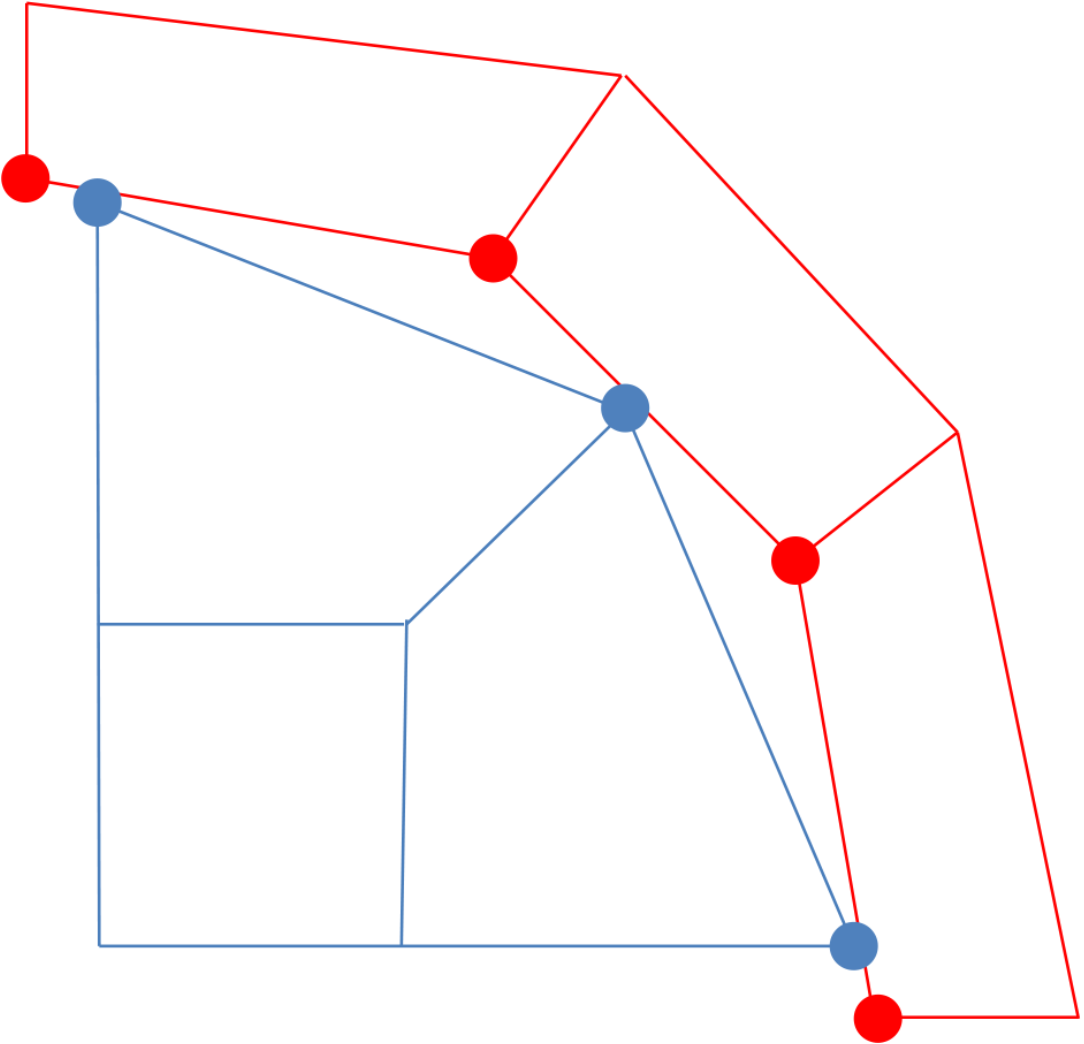 (b) Geometry after overlap removal.
Fig. 8.19 Effect of overlap removal on model geometry.
The process used to remove the initial overlap for three-dimensional solid elements involves changing the original coordinates of nodes on contact surfaces. Moving these coordinates yields a new mesh with the overlap removed; the overlap removal adds no initial stresses. Normal and tangential tolerances specific to overlap removal may be specified by the user for all contact surfaces in the REMOVE INITIAL OVERLAP command block. It is also possible to specify overlap normal and tangential tolerances on each surface pairing separately by using the INTERACTION command block. Overlap removal tolerances specified in INTERACTION command blocks will overwrite the tolerances specified in the REMOVE INITIAL OVERLAP command block. See Section 8.6.2 for details. The REMOVE INITIAL OVERLAP command block only removes overlaps that are detected among the surfaces and elements defined for contact, not all surfaces in the mesh. Overlap removal tolerances will be set automatically if no specific tolerances are given.
Overlap tolerances are used to designate a maximum amount of overlap to search for and remove. If the amount of overlap in the mesh is larger than those tolerances, then the overlap will not be found and removed.
The mesh modification done by the overlap removal feature changes the meshed geometry; therefore, also changing the mass and time step of affected elements. The modified mesh is returned in the results file and should be checked to ensure that the modifications are acceptable.
For some mesh geometries, especially for those where two mesh blocks have a large discrepancy in mesh size, overlap removal can result in poor element shapes and even “mushroomed” elements that appear to have squeezed out from between the blocks. A new command SETTINGS = OLD|IMPROVED(OLD) has been provided to help remedy this. The IMPROVED setting will increase the search tolerance and changes the interaction behavior to a tied friction model instead of a normal friction model. The default is SETTINGS = OLD.
8.9.4.1. Overlap Removal Diagnostics
The log file will contain a listing for maximum remaining overlap detected in the model after each overlap iteration. This maximum remaining overlap number should drive to zero over the overlap removal iterations. The code will output a warning if any initial overlap still exists after the overlap removal algorithms complete all iterations. Some initial overlap may still exist if there was excessive overlap in the initial configuration that could not be removed without inverting elements, or if there exists some pathology in the model geometry that the overlap removal algorithm cannot repair.
The log file contains two tables that relate to overlap removal. The first table lists the maximum amount any node of each block has been moved as a result of overlap removal. This quantity can be viewed on the mesh on a node by node basis by plotting the REMOVED_OVERLAP nodal variable on the results file. The second table lists the approximate maximum amount of overlap that exists in any element at the end of the overlap removal process. This variable can can be viewed on the mesh on an element by element basis by plotting the OVERLAP_VOLUME_RATIO element variable on the results file.
Note the remaining overlap value reported in the overlap removal iterations is computed in a slightly different way then the final overlap reported by the overlap volume ratio table. The overlap iteration number if based on surface intersections and nodal coordinates. The overlap volume ratio number is based on block volumes. The overlap volume ratio will detect overlaps such as whole volumes covering the same space that are not detected by the surface based algorithm. However, the overlap volume ratio also treats edge on edge overlaps and warped faces slightly differently than the surface based algorithm. As a result, small overlap volume ratios may be reported in a mesh even after the overlap removal algorithm completes successfully. If the overlap iterations drive the reported overlap to zero and the overlap volume ratio is some small number (generally one percent or lower) then the overlap removal algorithm was successful and all overlap was removed. Also note that the overlap removal algorithm will not remove overlap between bodies not in contact. The overlap volume ratio report will however still report overlaps for such bodies. Overlap of non-contacting bodies usually will not cause issues for models but is still reported to the log file for completeness.
8.9.4.2. Overlap Removal Commands
The OVERLAP ITERATIONS sets the number of overlap iterations that will be performed. The default value for OVERLAP ITERATIONS is \(100\) and is usually sufficient to remove overlap. More iterations may be able to remove more overlap. However, if the overlap cannot be completely removed in the default 100 iterations, it is likely that there is some model geometric pathology that cannot be resolved and additional iterations are unlikely to help. Overlap removal iterations may also be used after particle insertion, geometric disconnection, and other operations that modify the mesh topology. A high allowed iteration count can make these operations more expensive. An alternative use of the OVERLAP ITERATIONS command is to visualize initial input mesh overlap to help detect potential meshing or merging errors. If OVERLAP ITERATIONS is set to \(0\) overlap diagnostics will be computed but no overlap will be removed. Thus with zero overlap iterations output variables such as element overlap_volume_ratio will show the overlap metrics found in the initial unmodified mesh.
The DEBUG ITERATION PLOT command line allows visualization of the overlap removal iterations. Turning the command line on will print each overlap removal iteration to the results output file. The nodal variable “removed_overlap” can be used to show the progress of each overlap removal iteration. If the DEBUG ITERATION PLOT command is used after overlap removal, the analysis will terminate. Consequently, this command should only be used for debugging overlap removal.
The PRINT ALL DEBUGGING DATA command line allows all problematic overlap areas to be printed to the log file before exiting. By default, only a single problematic area is printed. Therefore, when debugging overlap issues, a simulation will need to be submitted multiple times. If this command is used, all information will be printed to the log file in the following fashion:
**  Error: Large amounts of overlap were found in the contact definition.
**  Overlaps were found in the following blocks:
**  block_1, block_2,
**  Element '22' on contact surface 'block_2' has 100.00% of its volume
**  overlapped by other elements.
**  This element is overlapped by the following:
**    Element           11 on contact surface 'block_1'
**    Element           10 on contact surface 'block_1'
**  Element '7' on contact surface 'block_1' has 97.92% of its volume overlapped
**  by other elements.
**  This element is overlapped by the following:
**    Element           17 on contact surface 'block_2'
**    Element           18 on contact surface 'block_2'
**    Element           19 on contact surface 'block_2'
The IGNORE KINEMATIC CONSTRAINTS command line allows one to ignore kinematic constraints during overlap removal iterations. By default, kinematic constraints such as fixed boundary conditions or prescribed velocities will be respected and enforced during overlap removal iterations. Nodes which have these constraints and are also overlapping cannot be moved from their prescribed locations, and thus can come into conflict with the overlap removal algorithm. When kinematic constraints exist on overlapping nodes, it is recommended to enable the IGNORE KINEMATIC CONSTRAINTS option to permit overlap removal on these nodes, or alternatively to fix the mesh overlap manually.
The REMOVE OVERLAP AT START OF TIME PERIODS command causes the overlap removal to be done at the start of each of the listed time periods. By default, overlap removal is done only at the start of the first time period. This command can be used to remove small overlaps between the pieces which are in contact before starting a new analysis time period.
Warning
Do not use REMOVE OVERLAP AT START OF TIME PERIODS, when having only one time period in your input file. In this case, this command is not needed and might cause unexpected behavior due to additional unnecessary overlap iterations.
If the OVERLAP REMOVAL ONLY = ON is used, the contact definition will only be used to remove initial overlap from the mesh. No contact enforcement will take place after overlap removal. This option can be used if it is desired for the overlap removal operations to use a different contact setup from the friction contact enforcement which is defined in a separate BEGIN CONTACT DEFINITION block.
8.9.4.3. Remove Initial Overlap Usage Guidelines
The following is a set of guidelines and restrictions which apply to overlap removal:
Overlap removal works only on the nodes which are part of the contact surfaces. This means overlap removal generally cannot successfully remove large amounts of overlap. Attempts to remove overlap of greater than half an element length may lead to inverted or poorly shaped elements, making further analysis impossible. In such cases, the large overlap needs to be removed manually by remeshing.
It is recommended to use the default normal and tangential tolerances for overlap removal whenever possible.
When working with lofted elements (shells, particles and beams) overlap removal may move the nodes of these elements, but will not change the lofted thickness of the elements.
Overlap removal only removes overlaps, it does not close initial gaps. Overlap removal attempts to bring overlapping surfaces exactly into contact but in some cases may result in small initial gaps between parts. However, for interactions that use the tied friction model and the line command
USE GAP REMOVAL = ON, initial gaps will be removed as well during overlap removal. See Section 8.5.5.Overlap removal will not move nodes that are kinematically constrained (such as nodes with fixed displacement boundary conditions).
When removing a gap at an interface, overlap removal will generally move both sides of that interface by equal amounts.
A tied contact friction model will work without overlap removal. However, it is still preferable to use overlap removal with tied contact as exactly matching interfaces lead to more accurate constraints.
When restarting an analysis, overlap removal is not applied to the restarted mesh. It is assumed that the restarted mesh is already in the proper configuration for contact.
8.9.5. Lofted Surface Options
Elements such as shells, beams, and particles are represented for contact with lofted geometry, which defines a geometric volume around these lower dimensional elements. This volume allows for contact to be unambiguously evaluated, so that situations such as stacked shells or edge on edge contact of shells can be handled naturally. Block skinning creates lofted geometry by default out of all shell, beam, and particle element blocks. Certain features of the lofted geometry may be controlled with the SURFACE OPTIONS command block.
BEGIN SURFACE OPTIONS
  SURFACE = <string list>surface_names
  REMOVE SURFACE = <string list>removed_surface_names
  BEAM RADIUS = <real>beam_radius
  LOFTED BEAM SHAPE = {HEXAGON|OCTAGON|SQUARE|HEXAGON_OUTER|OCTAGON_OUTER|SQUARE_OUTER}(HEXAGON)
  PARTICLE RADIUS = <real>part_radius
  LOFTED PARTICLE SHAPE = {CUBE|ICOSAHEDRON|OCTAHEDRON|TETRAHEDRON|
    PARENT_ELEMENT|SPHERE} (ICOSAHEDRON)
  CONTACT SHELL THICKNESS =
    ACTUAL_THICKNESS|LET_CONTACT_CHOOSE(ACTUAL_THICKNESS)
  ALLOWABLE SHELL THICKNESS TO ELEMENT SIZE RATIOS =
    <real>lower_bound(0.1) TO <real>upper_bound(1.0)
  SHELL CONTACT LOFTING FACTOR = <real>loftFactor
  SHELL CONTACT THICKNESS = <real>thickness
  CONTACT SHELL THICKNESS SCALE FACTOR = <real>scale_factor
  COINCIDENT SHELL TREATMENT = <string>
    DISALLOW|IGNORE|BEST(BEST)
  COINCIDENT SHELL HEX TREATMENT = <string>
    DISALLOW|IGNORE|TAPERED(TAPERED)
END [SURFACE OPTIONS]
The SURFACE and REMOVE SURFACE command lines specify which contact surfaces this command block refers to. These command lines are optional; by default the commands in the surface options block apply to all contact surfaces. If the SURFACE command line is used by itself, only those surfaces listed will be affected. If the REMOVE SURFACE command line is used by itself, all contact surfaces except those listed will be affected. Note, the surface names used in this command block are the names of the contact surfaces, not the names of the sidesets or blocks used to form those contact surfaces. Also, lofting is not performed on contact surfaces defined from sidesets; a warning will be thrown and the sidesets will not be lofted. To loft shells, the contact surfaces must be defined by blocks.
Warning
To loft shells for contact, the contact surfaces must be defined by blocks.
8.9.5.1. Lofted Beams
By default, contact represents the cross section of lofted beam elements by a six sided prism. The radius of the vertexes of the hexagons is the square root of the beam cross sectional area divided by pi. That is, the beam cross sectional area is converted into a circle, and then the hexagon end cap of the beam roughly represents this circle. Note that for a circular beam, the contact representation of that beam will nearly match the actual beam geometry. However, for an I-Beam cross section, the shape of the contact representation may be significantly smaller than the actual cross section length scales. The representation of various beams in contact is shown in Fig. 8.20.
By default, the lofted beam geometry is created as the inscribed geometry within the circle. However, in some cases, such as using tied contact between parts with beams, it may be desirable to loft the beams to the outer geometry of the circle. This can be achieved using the SQUARE_OUTER, HEXAGON_OUTER, and OCTAGON_OUTER options. If these options are not used, gaps may be present between the lofted geometry. See Fig. 8.21 below for a comparison of the options.
If a T AXIS command is given in a beam section the orientation of the lofted contact beam prism will be informed by that \(t\)-axis. Specifically one of the flat sides of the prism will be placed perpendicular to the beam \(t\)-axis. If no \(t\)-axis is given in the beam section the orientation of the beam prism will be arbitrary.
Lofted beam elements are used to represent beams, springs, dampers, and other one dimensional elements.
The BEAM RADIUS command can be used to explicitly set the radius of the lofted beam elements, overriding the default use of the beam’s cross sectional area.
The LOFTED BEAM SHAPE command changes how the beam is represented. Objects with fewer facets tend to be less accurate, but may run faster.
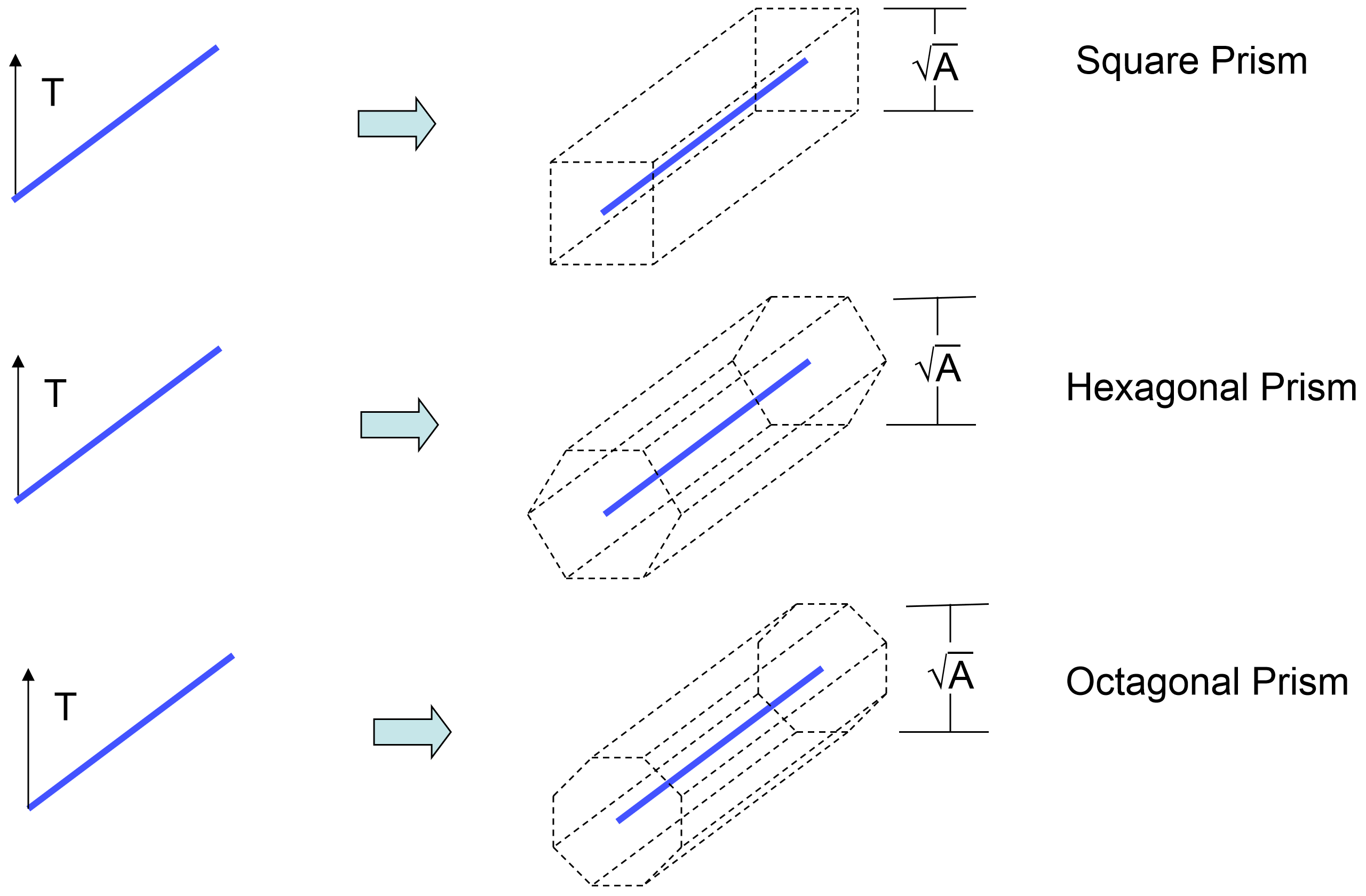
Fig. 8.20 Lofted beam geometry.
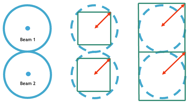
Fig. 8.21 Lofted beam demonstration, showing the difference between the default lofting and “OUTER” lofting.
8.9.5.2. Lofted Particles
The representation of various particles in contact are shown in Fig. 8.22. Lofted particle elements are used to represent mass particles, SPH particles, and other zero dimensional point elements.
The PARTICLE RADIUS command can be used to explicitly set the radius of the lofted particle elements. By default, lofted particles are represented as twenty-sided icosahedra having radii equal to the value of the element geometric_radius field.
The LOFTED PARTICLE SHAPE can change how finely the particle sphere is represented. Objects with fewer facets tend to be less accurate, but may result in improved run times. Note, the PARENT_ELEMENT option is experimental and only available for hexahedral elements converted to particles at initialization.
The LOFTED PARTICLE SHAPE = SPHERE command lofts an analytic sphere about the center or each particle instead of a twenty-sided icosahedron. The surface of the sphere defined by the particle radius is used in the closest point projection calculation. The closest point projection routine is then computed as normal. This option is expected to perform better for both accuracy and performance due to the spherical representation.
Warning
The LOFTED PARTICLE SHAPE = SPHERE command is only implemented for node-face contact.
Warning
When using this option, the particle block must be defined as the side B in the interaction definition.
Warning
Self contact is not yet implemented for this option. Self contact will function, but contact will create an interaction between the side B analytic sphere and the side A icosahedron particle. Performance benefits are still expected with this option, but not as drastic as self analytic sphere contact.
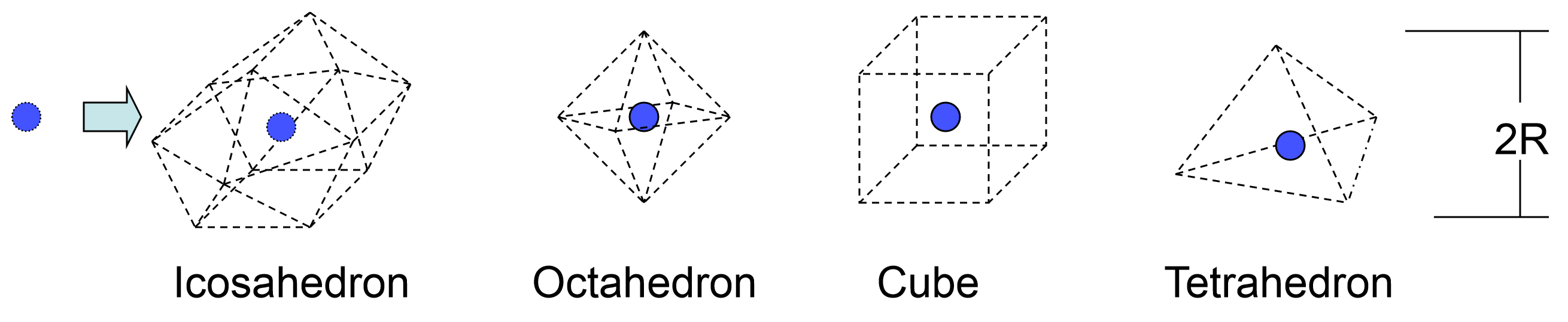
Fig. 8.22 Lofted particle geometry.
8.9.5.3. Lofted Shells
Lofted shells are represented by prisms around each shell element. An example representation of shells in contact is shown in Fig. 8.23. Lofted shells are used to represent shells, membranes, and other two dimensional elements. The lofted shell geometry is also based on the element section LOFTING FACTOR as shown in Fig. 6.4.
The CONTACT SHELL THICKNESS command line controls whether lofted shell contact uses the actual thickness of shell elements or a pseudo thickness that is computed by the contact algorithm. The default option to this command, ACTUAL_THICKNESS, causes the actual element thickness to be used. The LET_CONTACT_CHOOSE option to the CONTACT SHELL THICKNESS command tells the contact algorithm to create lofted geometries of the shells that are more appropriate for contact.
Shell elements that are very thick or very thin in relation to their in-plane dimension can be problematic in contact. A shell is considered very thin when the shell thickness is less than ten percent of the shell element’s in plane size. Thin shells may require a larger number of sub-steps in the contact algorithm to ensure that objects do not pass completely through the shell in a single step, causing contact to be missed. For thick shells, particularly near corners, the exterior geometry of these prisms may become jagged and not representative of the actual shell geometry. A shell may be considered very thick when the shell thickness is greater than the shell element’s in plane size.
Shell elements that are thick in relation to their in-plane dimension can produce ill-defined geometries, as seen in Fig. 6.4. The LET_CONTACT_CHOOSE option can help alleviate issues related to thick or thin shells. By default, when the LET_CONTACT_CHOOSE option is used, lofted geometry thicknesses are ensured to be within 0.1–1.0 times the in-plane dimension of the shell element. If the contact-appropriate shell thickness is computed to be outside of these bounds, the lofted shell thickness will be set to the upper or lower bound as appropriate.
The permissible bounds for the ratios of contact-appropriate thickness to actual thickness can be set using the lower_bound and upper_bound parameters in the ALLOWABLE SHELL THICKNESS TO ELEMENT SIZE RATIOS command. The ALLOWABLE SHELL THICKNESS command is functional only for Dash contact.
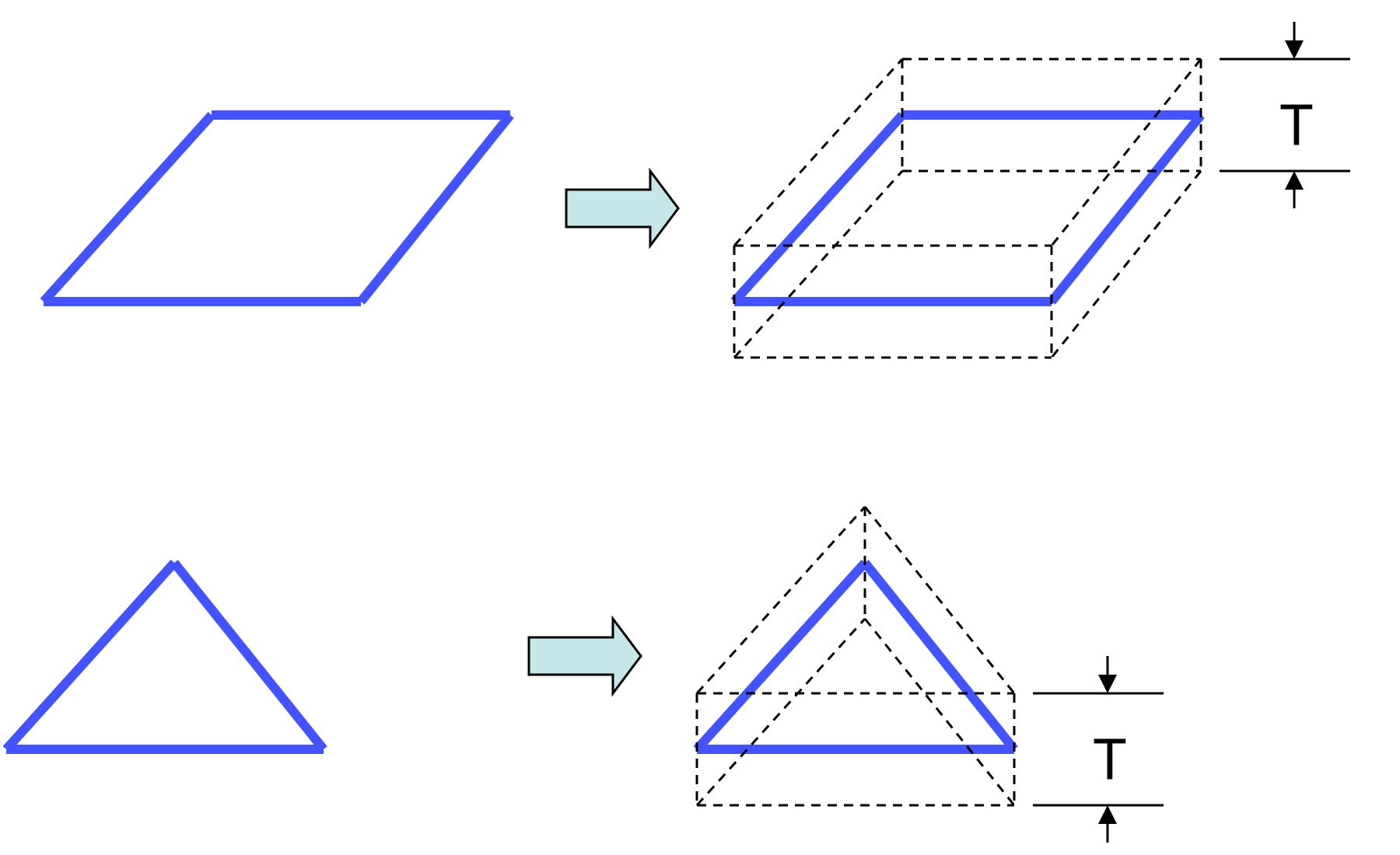
Fig. 8.23 Lofted shell geometry.
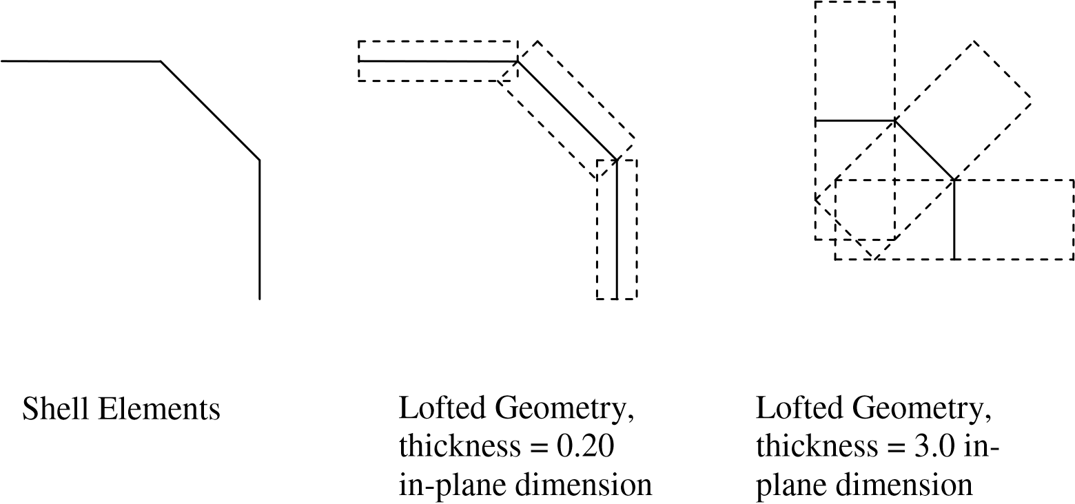
Fig. 8.24 Example lofted geometries produced by shell lofting.
A contact specific lofting factor for shells in can be set with the SHELL CONTACT LOFTING FACTOR command. For a description of shell lofting conventions see Section 6.2.5. By default contact uses the same lofting factor as does the shell element mechanics to loft the volume of the shell away from the shell element. The SHELL CONTACT LOFTING FACTOR will change the lofting factor for the shell in the contact algorithm, but not affect the lofting factor used for the element mechanics. This contact shell lofting factor can be used to properly fit together shell meshes without the algorithmic time step and stability limitations that can come from the lofting of the element mechanics.
A contact specific thickness for shells can be set with the SHELL CONTACT THICKNESS command. By default contact uses the same thickness as does the shell element mechanics. Note, this command overrides the ALLOWABLE SHELL THICKNESS TO ELEMENT SIZE RATIO option and explicitly sets an absolute contact thickness.
Additionally, the shell contact thickness can be set via the CONTACT SHELL THICKNESS SCALE FACTOR command. If this command is specified, the shell contact thickness well be set to the thickness used for the shell element mechanics multiplied by this scale factor. If both CONTACT SHELL THICKNESS SCALE FACTOR and SHELL CONTACT THICKNESS are specified for a surface, the SHELL CONTACT THICKNESS is used. Note, this command overrides the ALLOWABLE SHELL THICKNESS TO ELEMENT SIZE RATIO option and explicitly sets an absolute contact thickness.
8.9.5.4. Coincident Face Options
The COINCIDENT SHELL TREATMENT and COINCIDENT HEX SHELL TREATMENT command line identifies how elements that share the same nodes should be treated. This includes stacked shells and shell-clad faces of the hexahedral element. The default BEST allows coincident shells. The other options DISALLOW and IGNORE are provided for backwards compatibility.
If the DISALLOW option is selected then any time that coincident contact faces are found the code will abort with an error message indicating which elements were found to be coincident. The DISALLOW option should be used if you do not want any coincident shells to be considered in the analysis. The option operates essentially as a check on the mesh.
If the IGNORE option is selected, any contact faces attached to coincident shells or coincident shell/hexahedral boundaries are ignored for contact.
The default BEST and TAPERED options indicate that dash should use its standard shell lofting logic on coincident shells. For stacked shells this effectively means the shell stack has a contact thickness governed by the thickest shell in the stack. For coincident shell/hexahedral boundaries contact will be done on the shell faces which may be lofted somewhat away from the hexahedral face.
8.9.6. Search Options
BEGIN SEARCH OPTIONS [<string>name] # # Search tolerances NORMAL TOLERANCE = <real>norm_tol TANGENTIAL TOLERANCE = <real>tang_tol CAPTURE TOLERANCE = <real>cap_tolTENSION RELEASE = <real>ten_release
Contact involves a search phase and an enforcement phase. The contact search algorithm used to detect interactions between contact surfaces is often the most computationally expensive part of an analysis. The user can exert some control over how the search phase is carried out via the SEARCH OPTIONS command block. By selecting different options in this command block, the user can make trade-offs between the accuracy of the search and computing time.
The SEARCH OPTIONS command block begins with the input line:
BEGIN SEARCH OPTIONS [<string>name]
and ends with:
END [SEARCH OPTIONS <string>name]
The name for the command block is optional.
Without a SEARCH OPTIONS command block, the default search with associated default search parameters is used for all contact pairs. If you want to override the default search method for all contact pairs, you should add a SEARCH OPTIONS command block. By adding a SEARCH OPTIONS command block, you establish a new set of global defaults for the search for all contact pairs.
The valid command lines within a SEARCH OPTIONS command block are described in Section 8.9.6 and Section 8.9.6.1. The values specified by these commands are applied by default to all interaction contact surfaces, unless overridden by a specific interaction definition.
8.9.6.1. Search Tolerances
NORMAL TOLERANCE = <real>norm_tol
TANGENTIAL TOLERANCE = <real>tang_tol
As indicated previously, the contact functionality in Sierra/SM uses a box defined around each face to locate nodes that may potentially contact the face. This box is defined by a tolerance normal to the face and another tolerance tangential to the face (see Fig. 8.25). The code adds to these tolerances the maximum motion over a time step when identifying interactions. In the above command lines, the parameter norm_tol is the normal tolerance (defined on the NORMAL TOLERANCE command line) for the search box and the parameter tang_tol is the tangential tolerance (defined on the TANGENTIAL TOLERANCE command line) for the search box.
By default, Sierra/SM will automatically calculate normal and tangential tolerances roughly based on the characteristic length of a face multiplied by the value input by the search length scaling. The default search length scaling is \(0.15\). The automatic tolerances add the maximum motion over a time step just like the user defined tolerances. If you leave automatic search on and also specify normal and/or tangential tolerances with the NORMAL TOLERANCE and TANGENTIAL TOLERANCE command lines, the larger of the two (automatic or user specified) tolerances will be used. For example, suppose you specify a normal tolerance of \(1.0\times10^{-3}\) and the automatic tolerance computes a normal tolerance of \(1.05\times10^{-3}\). Then Sierra/SM will use a normal tolerance of \(1.05\times10^{-3}\).
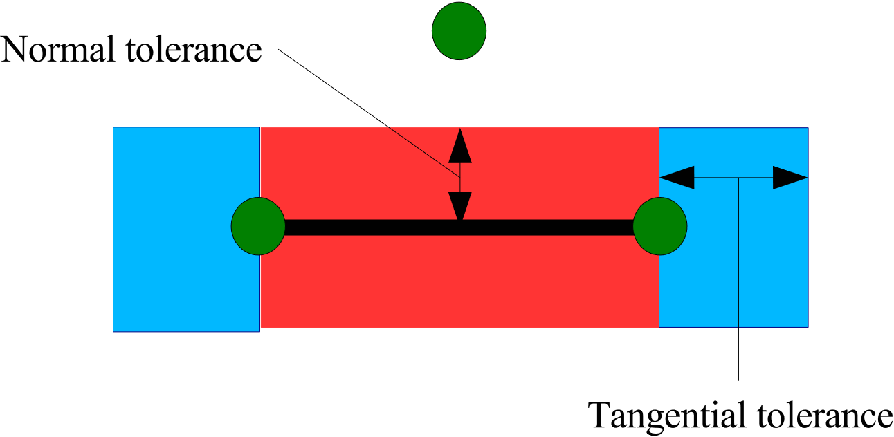
Fig. 8.25 Illustration of normal and tangential tolerances.
Both of these tolerances are absolute distances in the same units as the analysis. The proper tolerances are problem dependent. If a normal or tangential tolerance is specified in the SEARCH OPTIONS command block, they apply to all interactions. These default search tolerances can be overwritten for a specific interaction by specifying a value for the normal tolerance and/or tangential tolerance for that interaction inside the INTERACTION command block (see Section 8.6.2).
Normal and tangential contact tolerances are generally robustly automatically set and manual setting of tolerances should be avoided. If specific normal and tangential tolerances are set the tolerances used should not exceed roughly half of the minimum characteristic face size. Tolerances beyond that length may cause instability in the contact solution.
8.9.7. Enforcement Options
BEGIN ENFORCEMENT OPTIONS [<string>name]
  MOMENTUM BALANCE ITERATIONS = <integer>num_iterations(5)
  NUM GEOMETRY UPDATE ITERATIONS =<integer>num_updates(1)
  ACCUMULATED GAP REMOVAL OPTION =
    REMOVE_ALL|REMOVE_DEFAULT| REMOVE_NONE(REMOVE_DEFAULT)
END [ENFORCEMENT OPTIONS <string>name]
Contact involves a search phase to create constraints and an enforcement phase to enforce those constraints. The user can exert some control over how the enforcement phase is carried out via the ENFORCEMENT OPTIONS command block. By selecting different options in this command block, the user can make trade-offs between solution accuracy and computing time. The ENFORCEMENT OPTIONS command block begins with the input line:
BEGIN ENFORCEMENT OPTIONS [<string>name]
and is terminated with the input line:
END [ENFORCEMENT OPTIONS <string>name]
The name for the command block, name, is optional
Only a single ENFORCEMENT OPTIONS command block is permitted within a CONTACT DEFINITION command block. Without an ENFORCEMENT OPTIONS command block, the default enforcement algorithm with associated default enforcement options is used for all contact pairs. If you want to override the defaults for enforcement for all contact pairs, you should add an ENFORCEMENT OPTIONS command block. By adding this command block, you establish a new set of global defaults for enforcement for all contact pairs.
In DASH contact enforcement, equal and opposite forces are always applied to the nodes, preserving the momentum by construction. DASH then iterates on the gap between the side A and side B surfaces, minimizing the gap as much as possible. In DASH contact, the MOMENTUM BALANCE ITERATIONS command line specifies how many iterations to take to incrementally modify the forces to drive the gap to zero. In implicit contact, AL updates are a similar concept to momentum balance iterations. Note that in implicit, contact enforcement will be called as many times as needed to get below the residual values specified in the control contact block within the solver. Once the implicit contact solution is converged, the model problem will be updated with the nodal forces and positions predicted in contact.
For explicit contact, the number of passes (iterations) is set by the value num_iterations in the MOMENTUM BALANCE ITERATIONS command line. The default value for the number of iterations is 5. This value is generally acceptable for satisfying the material interpenetration constraint. To get accurate results in a global sense in analyses that use friction, a value of 10 is more appropriate. To get accurate contact response at individual points in analyses with friction, a value of 20 or greater may be needed. Note that as the number of iterations increases, the expense of enforcement increases. Thus a user can balance execution speed and accuracy with this command line, though care must be taken to ensure that the appropriate level of accuracy is attained. This command line affects only the enforcement phase of the contact. A single search phase is used for contact detection, but the enforcement phase uses an iterative process. Note that when using momentum balance iterations, only the contact forces and nodal coordinates are updated on the nodes in contact. The internal and external forces are not re-computed, and the other nodes not in contact are not updated until the next explicit timestep.
The NUM GEOMETRY UPDATE ITERATIONS defines the number of times contact will be enforced, updating the position of the current coordinates each iteration. By default, explicit contact uses one geometry update iteration. In an explicit step, first nodes move as if they have zero contact force; contact constraints are defined in this deformed configuration. Next, contact force is computed to enforce the constraints, remove interpenetration, satisfy friction laws, and compute a new deformed end of step state from the combination of contact, internal, and external forces. With additional geometry update iterations, the constraint equations are re-found in this updated configuration and then enforced again. Geometry update iterations can improve accuracy and stability if there is substantial motion over a single explicit time step. This can occur in hyper-velocity impact problems or if contact pressures are extremely high. However, geometry update iterations are very expensive. Taking two geometry update iterations will double the cost of contact.
The ACCUMULATED GAP REMOVAL OPTION controls how the explicit contact algorithm deals with either initial or accumulated gap in the frictionless and coulomb friction sliding interactions. Consider a mesh with initial overlap between contacting bodies. If the OVERLAP REMOVAL is not done then this initial overlap will be removed via standard contact forces. The ACCUMULATED GAP REMOVAL OPTION command will affect this case as follows:
The
REMOVE_ALLoption will remove all this existing gap over a single time step. The acceleration and force required to do this removal over the single explicit step may be very high, and may add a lot of energy to the system. The remove all option will tend to prevent any overlap from ever occurring in the mesh, but can lead to spuriously high energy and contact stability problems in some cases. Note, theREMOVE_ALLoption was the default interaction behavior before the 4.38 code release.The
REMOVE_NONEwill not remove any of the old gap. The contact constraint zero gap point will be defined with respect to the initial configuration. Thus the initial gap will not be removed and the initial overlap will not add energy. However, with theREMOVE_NONEoption it is possible for small errors in enforcement to accumulate gap in the interactions over time, this can lead to contact interactions being lost and bodies passing through one another.The
REMOVE_DEFAULTuses a heuristic weighting to remove some of the preexisting gap. The portion of preexisting gap removed will depend on the current gap and gap rate. Generally enough gap will be removed to ensure that accumulation of error will not cause loss of the interaction while the energy gain from preexisting gap removal is minimized. Preexisting gaps will be removed over several time steps. The default option provides a good balance of stability and contact accuracy and should be used for most circumstances.
Note, in addition to initial overlap preexisting gap can occur in many other circumstances including element death, particle creation, non-exact contact enforcement, and a variety of geometric ambiguities that can occur at corners. Thus selection of the gap removal option will have some, though generally minimal, effect on most runs.