9.16. J-Integral

Sierra/SM provides a capability to compute the \(J\)-integral via a domain integral.

Known Issue

Currently, the \(J\)-Integral evaluation capability is based on assumptions of elastostatics and a stationary crack, and is only implemented for 8-noded hexahedral elements with a single integration point.

\(J\) is analogous to \(G\) from linear elastic fracture mechanics (\(-\delta \pi / \delta a\)) and is the driving force on the crack tip of length \(a\) [[1], [2]]. Crack propagation occurs when \(J(a) \ge R(a)\), where \(R(a)\) is the material resistance. For constant \(R\), the resistance is often termed \(J_{c}\). In the reference configuration, the vector form of the \(J\)-integral in finite deformation [[3]] is

(9.2)\[\mathbf{J}=\int_{\Gamma_{0}}{\boldsymbol{\Sigma}\mathbf{N}\,\text{d}A}\]

where \(\boldsymbol{\Sigma} = W\mathbf{I} - \mathbf{F}^{T}\mathbf{P}\) is called the Eshelby energy-momentum tensor [[4]]. \(W\) is the stored energy density in the reference configuration and \(\mathbf{F}\) and \(\mathbf{P}\) are the deformation gradient and first Piola-Kirchhoff stress, respectively. Rice [[2]] realized that because \(\boldsymbol{\Sigma}\) is divergence-free in the absence of body forces, one can examine \(\mathbf{J}\) in the direction of the defect \(\mathbf{L}\) (unit vector) and obtain a path-independent integral for traction-free crack faces. \(J\) can be written as

(9.3)\[J=\int_{\Gamma_{0}}{\mathbf{L} \cdot \boldsymbol{\Sigma}\mathbf{N}\,\text{d}A}\]

and interpreted as a path-independent driving force in the direction of the defect. We note that one can also express \(\boldsymbol{\Sigma}\) in terms of \(\bar{\boldsymbol{\Sigma}}\), where \(\bar{\boldsymbol{\Sigma}} = W\mathbf{I} - \mathbf{H}^{T}\mathbf{P}\) and \(\mathbf{H} = \text{Grad}\,\mathbf{u}\). Although \(\boldsymbol{\Sigma}\) is symmetric and \(\bar{\boldsymbol{\Sigma}}\) is not symmetric, they are equivalent when integrated over the body (\(\text{Div}\mathbf{P}=\mathbf{0}\)). Differences in the energy-momentum tensor stem from the functional dependence of the stored energy function \(W\). \(\boldsymbol{\Sigma}\) and \(\bar{\boldsymbol{\Sigma}}\) derive from \(W(\mathbf{F})\) and \(W(\mathbf{H})\), respectively. When integrated, both collapse to the familiar 2-D relation for infinitesimal deformations.

(9.4)\[J=\int_{\Gamma}{\mathbf{e}_{1} \cdot \boldsymbol{\Sigma}\mathbf{n}\,\text{d}s} = \int_{\Gamma}{(Wn_1-u_{i,1}\sigma_{ij}n_j)\text{d}s}\]

9.16.1. Technique for Computing J

\(J\) is often expressed as a line (2D) or surface (3D) integral on a ring surrounding the crack tip. Defining a smooth ring over which to compute this surface integral and performing projections of the required field values onto that ring presents many difficulties in the context of a finite element code.

To compute the \(J\)-integral in a finite element code, it is more convenient to perform a volume integral over a domain surrounding the crack tip. We can then leverage the information at integration points rather than rely on less accurate projections. To do this, we follow the method described in [[5]]. We replace \(\mathbf{L}\) with a smooth function \(\mathbf{q}\). On the inner contour of the domain \(\Gamma_{0}\), \(\mathbf{q} = \mathbf{L}\). On the outer contour of the domain \(C_{0}\), \(\mathbf{q} = \mathbf{0}\). Because the outer normal of the domain \(\mathbf{M}\) is equal and opposite of the normal \(\mathbf{N}\) on \(\Gamma_{0}\), there is a change of sign. For traction-free surfaces, we can apply the divergence theorem, enforce \(\text{Div}\bar{\boldsymbol{\Sigma}}=\mathbf{0}\), and find that the energy per unit length \(\bar{J}\) is

(9.5)\[\bar{J}=-\int_{\Omega_{0}}(\bar{\boldsymbol{\Sigma}}:\text{Grad}\,\mathbf{q})\text{d}V.\]

We can also introduce a correction if we seek to consider cases in which the crack faces, \(A_{0}^{+} + A_{0}^{-}\), or “caps”, \(S_{0}^{+} + S_{0}^{-}\), of the domain are not traction free. For example, both cases would be satisfied for a thumbnail crack in a pressure vessel. The correction

(9.6)\[\bar{J}=-\int_{\Omega_{0}}(\bar{\boldsymbol{\Sigma}}:\text{Grad}\,\mathbf{q})\text{d}V- \int_{S_{0}^{+} + S_{0}^{-} + A_{0}^{+} + A_{0}^{-}}{\mathbf{q} \cdot \mathbf{H}^{T}\mathbf{T}\,\text{d}A}.\]

effectively removes the contribution of the applied tractions and ensures that the integral remains path independent. We note that the correction is integrated in the reference configuration with referential traction \(\mathbf{T}\). When pressure is applied to \(S_{0}^{+}\), \(S_{0}^{-}\), \(A_{0}^{+}\), or \(A_{0}^{-}\), Sierra employs (9.6).

We note that all the field quantities are given via simulation and we choose to define \(\mathbf{q}\) on the nodes of the domain \(\mathbf{q}^{I}\). We then employ the standard finite element shape functions to calculate the gradient. We can specify the crack direction \(\mathbf{L}\) or assume that the crack will propagate in the direction normalto the crack front \(-\mathbf{M}\). For a “straight” crack front, \(\mathbf{L} = -\mathbf{M}\). If \(\mathbf{S}\) is tangent to the crack front and \(\mathbf{T}\) is normal to the lower crack surface, \(\mathbf{S} \times \mathbf{M} = \mathbf{T}\). We note that for non-planar, curving cracks, \(\mathbf{M}\), \(\mathbf{S}\), and \(\mathbf{T}\) are functions of the arc length \(S\). For ease, we employ the notation \(\mathbf{N}\) rather than \(-\mathbf{M}\). For a crack front \(S_{0}\), we can define the average driving force \(J_{avg}\) as

(9.7)\[{J_{avg}}=\frac{\bar{J}}{\int_{S_{0}}\mathbf{L} \cdot \mathbf{N}\,\text{d}S}.\]

While the average driving force is useful for interpreting experimental findings and obtaining a macroscopic representation of the driving force, we also seek to examine the local driving force \(J(S)\). Using the finite element interpolation functions to discretize \(\mathbf{L}\) through the smooth function \(\mathbf{q}\), we find \(\mathbf{q} = \lambda^{I}\mathbf{q}^{I}\). For a specific node \(K\), we can define \(|\mathbf{q}^{K}| = 1\) and \(\mathbf{q}^{I} = \mathbf{0}\) for all other \(I \ne K\) on \(S_{0}\). Note that we still need to specify the function \(\mathbf{q}\) in the \(\mathbf{S}-\mathbf{T}\) plane from the inner contour \(\Gamma_{0}\) to the outer contour \(C_{0}\). The resulting expression for the approximate, point-wise driving force at node \(K\) on the crack front is

(9.8)\[J^{K}=\frac{\bar{J}}{\int_{S_{0}} \lambda^{K}\mathbf{q}^{K} \cdot \mathbf{N}\,\text{d}S}.\]

Again, we note that if the direction of propagation \(\mathbf{L}\) is taken in the direction of the normal \(\mathbf{N}\), the denominator is \(\int_{S_{0}} \lambda^{K}\text{d}S\). More information regarding the point-wise approximation of \(J^{K}\) can be found in [[6], [7]].

Additional information on the J Integral capability can be found in [[8]].

9.16.2. Input Commands

Output quantities related to \(J\)-integrals may be computed during the analysis by including one or more J INTEGRAL command blocks in the REGION scope. This block can contain the following commands:

BEGIN J INTEGRAL <jint_name>
  #
  # Definition of integration domain
  BLOCK = <string list>blockNames
  REMOVE BLOCK = <string list>removeBlocks
  ELEMENT = <int_list>elemNumbers
  ASSEMBLY = <string list>assemblyNames
  INCLUDE ALL BLOCKS
  #
  # integral parameter specification commands
  CRACK PLANE SIDE SET = <string list>side_sets
  CRACK TIP NODE SET = <string list>node_sets
  USE SURFACE FOR EDGE DIRECTION = OFF|ON(ON)
  CRACK DIRECTION = <real>dir_x
                    <real>dir_y
                    <real>dir_z
  INTEGRATION RADIUS = <real>int_radius
  NUMBER OF DOMAINS = <integer>num_domains
  FUNCTION =
     PLATEAU|PLATEAU_RAMP|LINEAR(PLATEAU)
  SYMMETRY = OFF|ON(OFF)
  DEBUG OUTPUT = OFF|ON(OFF) WITH
    <integer>num_nodes NODES ON THE CRACK FRONT
  #
  # time period selection commands
  ACTIVE PERIODS = <string list>period_names
  INACTIVE PERIODS = <string list>period_names
END J INTEGRAL <jint_name>

The \(J\)-integral is performed over a domain defined by a set of elements using the standard element assignment commands. See Section 7.1.1 for details.

A set of parameters must be provided to define the crack geometry used in the calculation of the \(J\)-integral. The \(J\)-integral command block uses a sideset on one surface of the crack plane behind the crack tip and a nodeset containing the nodes on the crack tip. Both the CRACK PLANE SIDE SET and CRACK TIP NODE SET commands are required. These commands specify the names of the sideset behind the crack tip and the nodeset on the crack tip, respectively. Assemblies may contain blocks, or assemblies of these.

By default, the direction of crack propagation is computed from the geometry of the crack plane and tip, as provided in the crack plane sideset and crack tip nodeset (\(\mathbf{L}=\mathbf{N}\)). At locations where the crack intersects a surface, the computed \(\mathbf{N}\) is commonly less accurate. At these locations, the USE SURFACE FOR EDGE DIRECTION = ON command will attempt to improve \(\mathbf{N}\) by projecting it onto the intersected surface. The default is ON, and USE SURFACE FOR EDGE DIRECTION = OFF should only be set if the crack tip is known to intersect the surface at a sharp angle. Alternatively, the CRACK DIRECTION command can be used to override the computed direction of crack propagation (\(\mathbf{L}\)). This command takes three real numbers that define the three components of the crack direction vector in the global XYZ coordinate system.

To fully define the domains used for the domain integrals, the radius of the domains and the number of domains must also be specified. A series of disc-shaped integration domains are formed with varying radii going out from the crack tip. The INTEGRATION RADIUS command specifies the radius of the outermost domain. The number of integration domains is specified using the NUMBER OF DOMAINS command. The radii of the domains increase linearly going from the innermost to the outermost domain. The domains will only include elements included in the overall integration domain defined by the BLOCK command and other related commands.

The weight function \(\mathbf{q}\) used to calculate the \(J\)-integral is specified by use of the FUNCTION command line. The LINEAR function sets the weight function to 1.0 on the crack front \(\Gamma_{0}\) and 0.0 at the edge of the domain \(C_{0}\), int_radius away from the crack tip. The PLATEAU function, which is the default behavior, sets all values of the weight function to 1.0 that lie within the domain of integration and all values outside of the domain are set to 0.0. This allows for integration over a single ring of elements at the edge of the domain. The third option for the FUNCTION command is PLATEAU_RAMP, which for a single domain will take on the same values as the LINEAR function. However, when there are multiple domains over the radius int_radius, the \(n^{th}\) domain will have weight function values of 1.0 over the inner \(n-1\) domains and will vary from 1.0 to 0.0 over the outer \(n^{th}\) ring of the domain. These functions can be seen graphically in Fig. 9.18.

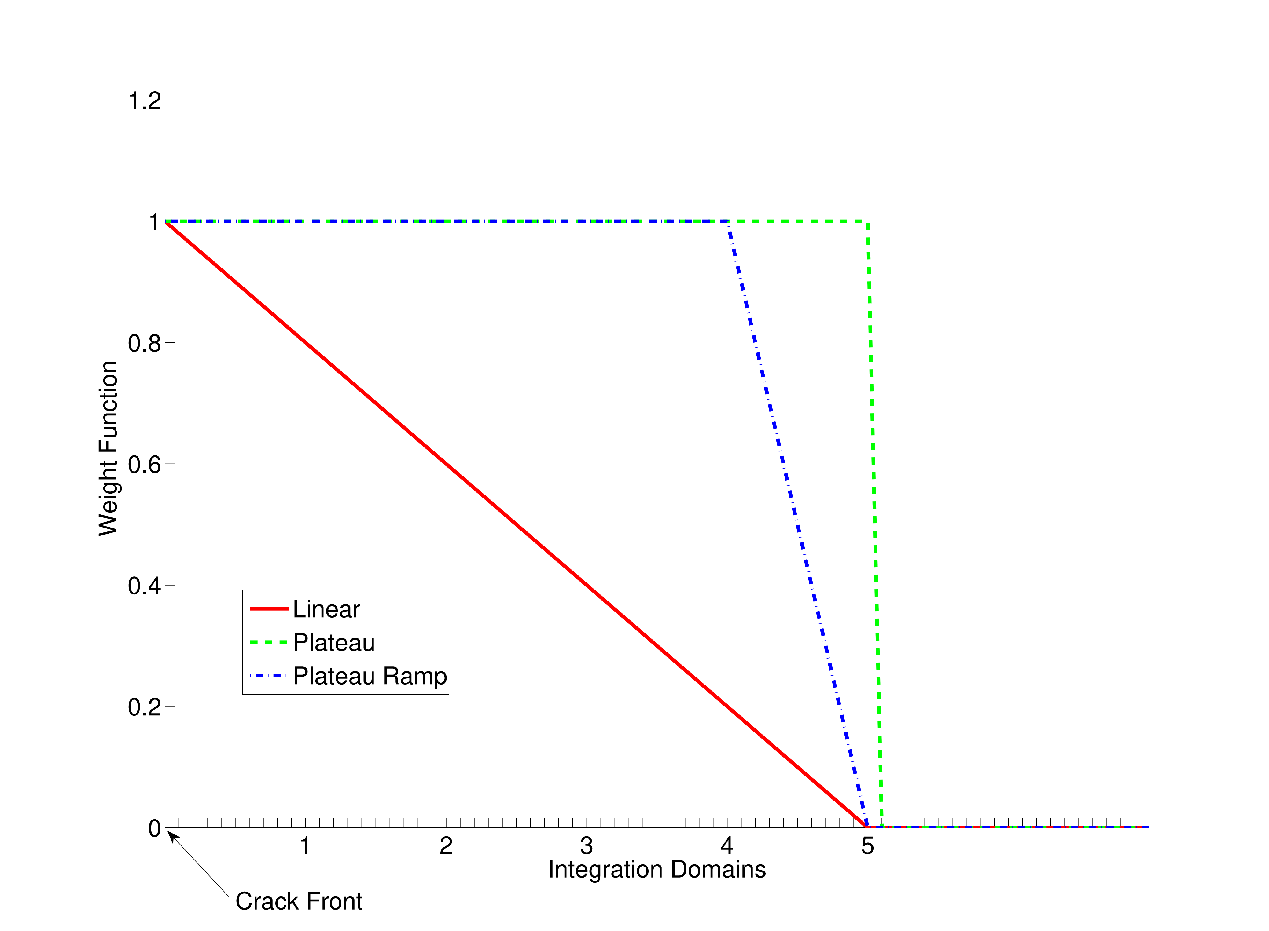
Fig. 9.18 Example weight functions for a \(J\)-integral integration domain. Weight functions shown for domain 5.

We note that in employing both the PLATEAU and the PLATEAU_RAMP functions, one is effectively taking a line integral at finite radius (albeit different radii). In contrast, the LINEAR option can be viewed as taking the \(lim \; \Gamma_{0} \rightarrow 0^{+}\). If the model is a half symmetry model with the symmetry plane on the plane of the crack, the optional SYMMETRY command can be used to include the symmetry conditions in the formation of the integration domains and in the evaluation of the integral. The default behavior is for symmetry to not be used.

The user may optionally specify the time periods during which the \(J\)-integral is computed. The ACTIVE PERIODS and INACTIVE PERIODS command lines are used for this purpose. See the Section 2.6 for more information about these command lines.

9.16.3. J-Integral Region

Optionally, a J_INTEGRAL REGION can be used for computation and output of \(J\)-integral quantities. This particular region must be part of an input deck with multiple regions: an ADAGIO REGION and the J_INTEGRAL REGION. The input deck structure is as follows.

BEGIN ADAGIO REGION <string>adagio_region_name
  USE FINITE ELEMENT MODEL <string>full_model_name
  # adagio commands for boundary value problem
  ...
END [ADAGIO REGION <string>adagio_region_name]

BEGIN J_INTEGRAL REGION <string>jintegral_region_name
  USE FINITE ELEMENT MODEL <string>refined_crack_model_name
  # one or more J-integral command blocks
  # output of J-integral fields
END [J_INTEGRAL REGION <string>jintegral_region_name]

The J_INTEGRAL REGION is essentially a post-processing region specifically designed for the \(J\)-integral capability. The usage of a separate region with the USE FINITE ELEMENT MODEL command line allows for a separate mesh to be used for the computation of the \(J\)-integral. This facilitates the ability to use a well-structured, highly refined hexahedral mesh of the crack for robust \(J\)-integral computations, while using a generally unstructured, less refined mesh with any three-dimensional solid element (textit{e.g.}, tetrahedra) for modeling the crack in the full model being analyzed. At every results output step in the J_INTEGRAL REGION, Sierra/SM performs an \(L_2\)-projection transfer (see Section 11.2) from the ADAGION REGION. This transfer includes all fields needed by the \(J\)-integral, and it is immediately followed by computation and output of the requested \(J\)-integral quantities. The transfer is fully automated and cannot be re-defined or modified in the input deck commands for the J_INTEGRAL REGION.

The only additional command block available in the J_INTEGRAL REGION is the pressure boundary condition (see Section 7.7.1). This boundary condition is available only for the purpose of allowing the \(J\)-integral algorithm to apply the appropriate pressure corrections. These pressure boundary conditions should identically match equivalent pressure boundary conditions applied in the ADAGIO REGION; the pressure magnitudes and surfaces receiving the pressure loads should be consistent between the two regions.

9.16.4. Output

Many variables are generated for output when the computation of the \(J\)-integral is requested. The average value of \(J\) for each integration domain is available as a global variable, as described in Table Table 9.27. The point-wise value of \(J\) at nodes along the crack for each integration domain is available as a nodal variable, as shown in Table Table 9.28. An element variable to illustrate the integration domains is also available, as listed in Table Table 9.29.

The DEBUG OUTPUT command is useful to generate output data for debugging the \(J\)-integral. If the DEBUG OUTPUT = ON|OFF(OFF) WITH <integer>num_nodes NODES ON THE CRACK FRONT line command is set to ON, the weight functions, \(q\), will be output for each node-based \(J\) value that is calculated. The user must specify num_nodes, which represents the number of nodes along the crack front. An internal check is performed during problem initialization that will verify that the number of nodes specified by the user on the command line matches the number of nodes associated with the crack front.

Warning

Using the DEBUG OUTPUT command line can potentially result in an extremely large output file because every node in the integration domain will now compute and store \((NumNodeOnCrackFront + 1)*NumDomains\) weight function vectors. This can also potentially exhaust the available memory on the machine.

9.16.5. Required Discretization

In order to enable the correct construction of the test function \(\mathbf{q}^{I}\), the hexahedral mesh should be orthogonal to the crack front. An orthogonal mesh will ensure that the elements are not skewed along the crack front. Because these elements will experience large deformation during crack-tip blunting, well-formed elements increase the accuracy of the solution. We note that this capability is not specific to crack front nodes. Any ellipsoidal surface with a constant bias will generate skewed elements.

In addition, an orthogonal mesh will ensure that the location of a point-wise surface integral will be a closest point projection from the crack-tip node. Consequently, any surface integral via a domain integral at a node along the crack front will be most accurate if the specified radius is a minimum. In addition to increasing the accuracy of point-wise evaluations of the \(J\)-integral, an orthogonal mesh will also ease the search algorithm for point-wise evaluations. The search is performed along the normal to the crack front. If the mesh is aligned with the normal, the specification of \(\mathbf{q}\) is straightforward. Misalignment can result in a “checker boarding” of the integration domains which presents the possibility that \(\mathbf{q}^{I}\) will always be one and the \(J\)-integral will be zero. Future work may generalize the calculation of \(J^{K}\), but we are currently limited to hexahedra. Given these requirements, we collaborated with the Cubit team to add the capability to generate meshes orthogonal to a surface. The Cubit team implemented the command

adjust boundary surface AA snap_to_normal curve A

which enables the generated elements on surface AA to be “snapped” normal to the curve A. For example, one may choose to sweep adjacent squares along the crack front curve A. For crack plane surfaces AA and AB joined by the crack front curve A, one would issue the following commands in Cubit

surface AA AB scheme map
mesh surface AA
node in curve A position fixed
adjust boundary surface AA snap_to_normal curve A
mesh surface AB
node in curve A position fixed
adjust boundary surface AB snap_to_normal curve A
          fixed curve A

to obtain an orthogonal mesh. The next step is to sweep that mesh “up” and “down” from the crack surface. To ensure that Cubit employs a “simple” sweep so that the search is consistent through the direction of the sweep, we use

volume ABC  scheme sweep source surface AA target
      surface AC
propagate_bias autosmooth_target off sweep_smooth
      linear
sweep_transform translate

for volume ABC. Because proper mesh construction ensures accuracy and smoothness in \(J^{K}\), we encourage analysts to use the snap_to_normal and autosmooth_target off options.

9.16.6. Results and History Output

This section lists output variables for \(J\)-Integral.

• Table Table 9.27 Global Variables for \(J\)-Integral

• Table Table 9.28 Nodal Variables for \(J\)-Integral

• Table Table 9.29 Element Variables for \(J\)-Integral

Table 9.27 Global Variables for \(J\)-Integral

Variable Name	Type	Comments
j_average_<jint_name>	Real[]	Average value of the \(J\)-integral over the crack. Array sized to number of integration domains and numbered from inner to outer domain. <jint_name> is the name of the J INTEGRAL block.

Table 9.28 Nodal Variables for \(J\)-Integral

Variable Name	Type	Comments
j_<jint_name>	Real[]	Point-wise value of \(J\)-integral along crack. Array sized to number of integration domains and numbered from inner to outer domain. <jint_name> is the name of the J INTEGRAL block.

Table 9.29 Element Variables for \(J\)-Integral

Variable Name	Type	Comments
j_integration_domains_<jint_name>	Integer[]	Flag indicating elements in integration domains. Set to 1 if in domain, 0 otherwise. Array sized to number of domains and numbered from inner to outer domain. <jint_name> is the name of the J INTEGRAL block.

---

[1]

J.D. Eshelby. The force on an elastic singularity. Philosophical Transactions of the Royal Society of London A, 244:87–112, 1951. doi:10.1098/rsta.1951.0016.

[2] (1,2)

J.R. Rice. A path independent integral and the approximate analysis of stress concentration by notches and cracks. Journal of Applied Mechanics, 35:379–386, 1968.

[3]

G.A. Maugin. Material Inhomogeneities in Elasticity. Chapman & Hall/CRC, New York, 1993.

[4]

J.D. Eshelby. Energy relations and the energy-momentum tensor in continuum mechanics. In M. Kannien, editor, Inelastic Behavior of Solids, pages 77–114. McGraw-Hill, New York, 1970.

[5]

F.Z. Li, C.F. Shih, and A. Needleman. A comparison of methods for calculating energy release rates. Engineering Fracture Mechanics, 21:405–421, 1985. doi:10.1016/0013-7944(85)90029-3.

[6]

C.F. Shih, B. Moran, and T. Nakamura. Energy release rate along a three-dimensional crack front in a thermally stressed body. International Journal of Fracture, 30:79–102, 1986. doi:10.1007/BF00034019.

[7]

ABAQUS. Theory Manual. Volume Version 6.7. Hibbitt, Karlsson and Sorensen, Providence, RI, 2007.

[8]

Y. Ohashi, J.W. Foulk, and A.J. Lindblad. Verification of J integral capability in sierra mechanics. Technical Report SAND2012-8720, Sandia National Laboratories, Albuquerque, NM, 2012.