7.8. Distributed Force and Moment

BEGIN DISTRIBUTED {FORCE|MOMENT}
  #
  # Node set commands
  NODE SET|NODESET = <string list>nodelist_names
  SURFACE|SIDESET|SIDE SET = <string list>surface_names
  BLOCK = <string list>block_names
  ASSEMBLY = <string list>assembly_names
  ELEMENT = <int list>elem_numbers
  NODE = <int list>node_numbers
  INCLUDE ALL BLOCKS
  REMOVE NODE SET = <string list>nodelist_names
  REMOVE SURFACE = <string list>surface_names
  REMOVE BLOCK = <string list>block_names
  #
  # Load definition commands
  SCALE FACTOR = <real>scale_factor(1.0)
  FUNCTION = <string>function_name
  DIRECTION = <string>defined_direction |
    !COMPONENT = <string>X|Y|Z
  COORDINATE SYSTEM = <string>sys_name(global)
  #
  # additional commands
  ACTIVE PERIODS = <string list>period_names
  INACTIVE PERIODS = <string list>period_names
END [DISTRIBUTED {FORCE|MOMENT}]

The distributed force and moment boundary conditions are used to apply a specific total net force or moment that is automatically distributed to a finite set of nodes. The distributed force and moment boundary conditions differ from the prescribed force Section 7.7.3 and moment Section 7.7.4 boundary conditions. The previously described prescribed force boundary conditions apply user defined point loads to each and every node used by the boundary condition. The distributed force BC instead spreads a single user defined target load among every node in the set. The distributed moments are applied via translational force couples and thus can be used on any element type. This differs from the prescribed point load moments Section 7.7.4 which can only be used on elements with rotational degrees of freedom such as shells.

The distributed load boundary conditions are targeted to the following types of use cases.

Apply a moment to a solid meshed body, for example torque on a shaft or bending moment on the end of a solid meshed bar.
Apply an exact known force to a model boundary. For example to model a load-control tension test.
Apply a load to known load to a model distributed over a finite volume. An analysis with this distributed load will converge with mesh refinement. An analysis with a concentrated load applied to a single point will generate a singularity at that point and not converge with mesh refinement.

7.8.1. Node Set Commands

The Node set commands portion of the DISTRIBUTED FORCE and DISTRIBUTED MOMENT command blocks define a set of nodes associated with the boundary condition. These command lines, taken collectively, constitute a set of Boolean operators for constructing a set of nodes. See Section 7.1.1 for more information about the use of these command lines. The boundary condition must contain at least one NODE SET|NODESET, NODE, SURFACE, BLOCK, ELEMENT, ASSEMBLY, or INCLUDE ALL BLOCKS command line. Note, the RIGID BODY command is not available with this boundary condition. Assemblies may contain blocks, surfaces, nodesets, or assemblies of these.

7.8.2. Load Definition Commands

The load commands define the magnitude and direction of the force or moment applied by the distributed load boundary condition. The load magnitude is defined by the time history function function_name multiplied by the value of scale_factor. Each distributed load BC takes a single load magnitude, the FUNCTION command by default takes a function of time and may also take a analytic function that involves other global variables. One and only one of the COMPONENT command line or DIRECTION command line must be given to define the load direction. For the distributed force BC the load will be in the given direction. For the distributed moment BC the load will be around the given direction using the right hand rule. If no coordinate system is given the direction or component refer to the global XYZ coordinate system. If an optional coordinate system is specified the directions and components are given with respect to that coordinate system. Note if the coordinate system is dynamic (linked to coordinates of node sets) the direction of distributed load application will update continuously as the model evolves.

7.8.3. Miscellaneous Commands

The ACTIVE PERIODS and INACTIVE PERIODS command lines provides an additional option for the distributed load BC. These command lines can activate or deactivate the load for certain time periods. See Section 2.6 for more information about these command lines.

7.8.4. Restrictions and Assumptions

The distributed load boundary conditions are applied by defining a set of translational forces on the nodes in the application region. Generally forces will be mass proportional. Example force distributions for Z force and Z moment are shown in Fig. 7.4 and Fig. 7.5. Force distributions are constructed to apply net load in only a single component. Thus the force distribution shown in Fig. 7.4 produces no net moment on the surface and no net Force in the X and Y directions. The moment distribution shown in Fig. 7.5 produces no net force on the surface nor any net moment around the X or Y axes.

As moments are constructed via translational force couples no net moment can be applied to a single node. Additionally if all the applied nodes fall nearly in a line no net moment can be applied around that line. If these degenerate cases occur the inapplicable component of the net moment will be zero. For node sets that are close to collinear potentially nonphysical large forces may be required to apply due to the small axial moment arm. When using the distributed moment BC generally the application region should be a fairly large set of nodes on a block or surface to prevent these excessive force concentrations.

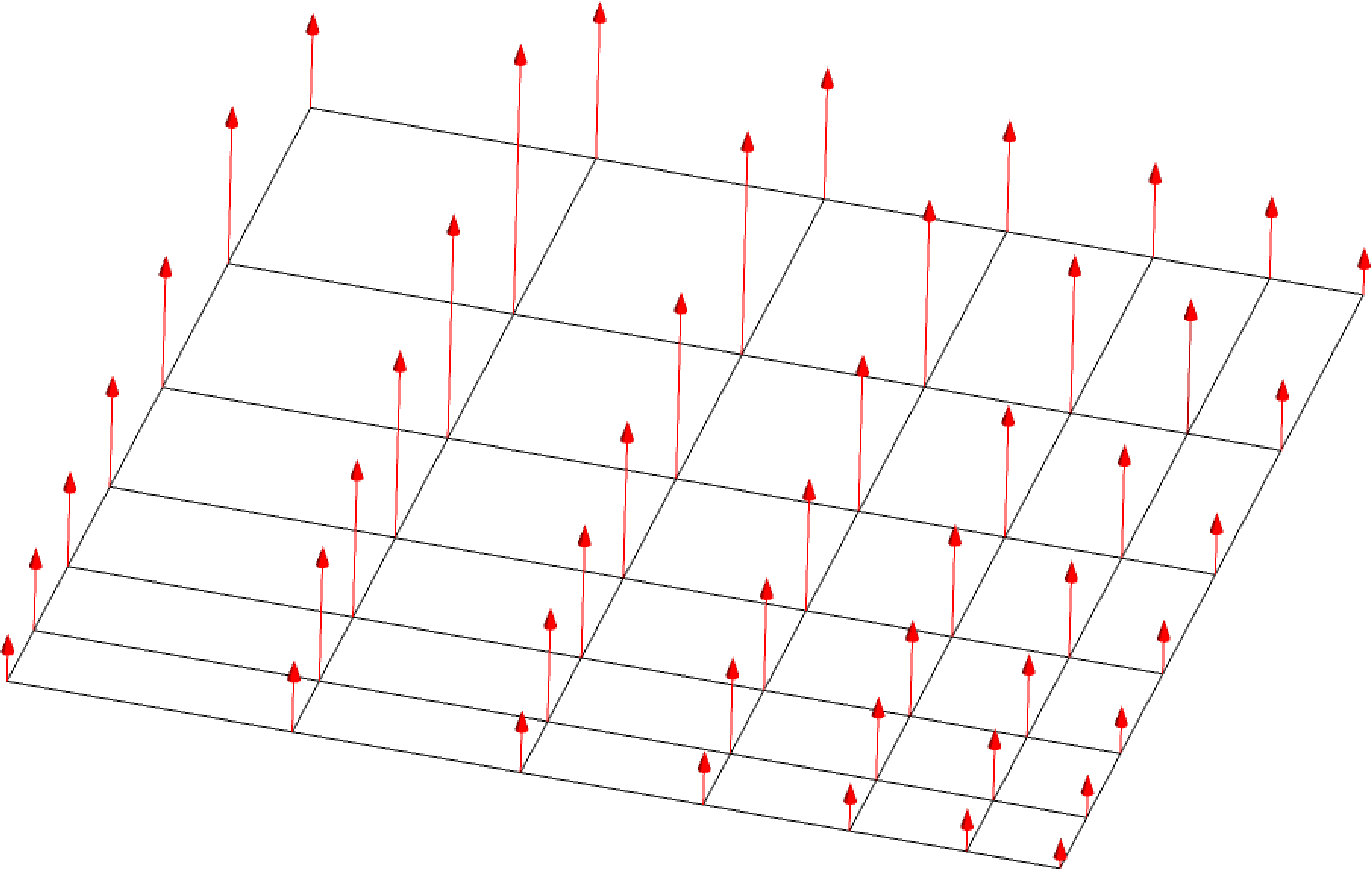
../../_images/Force_load.png — Fig. 7.4 Distributed Z force load distribution.

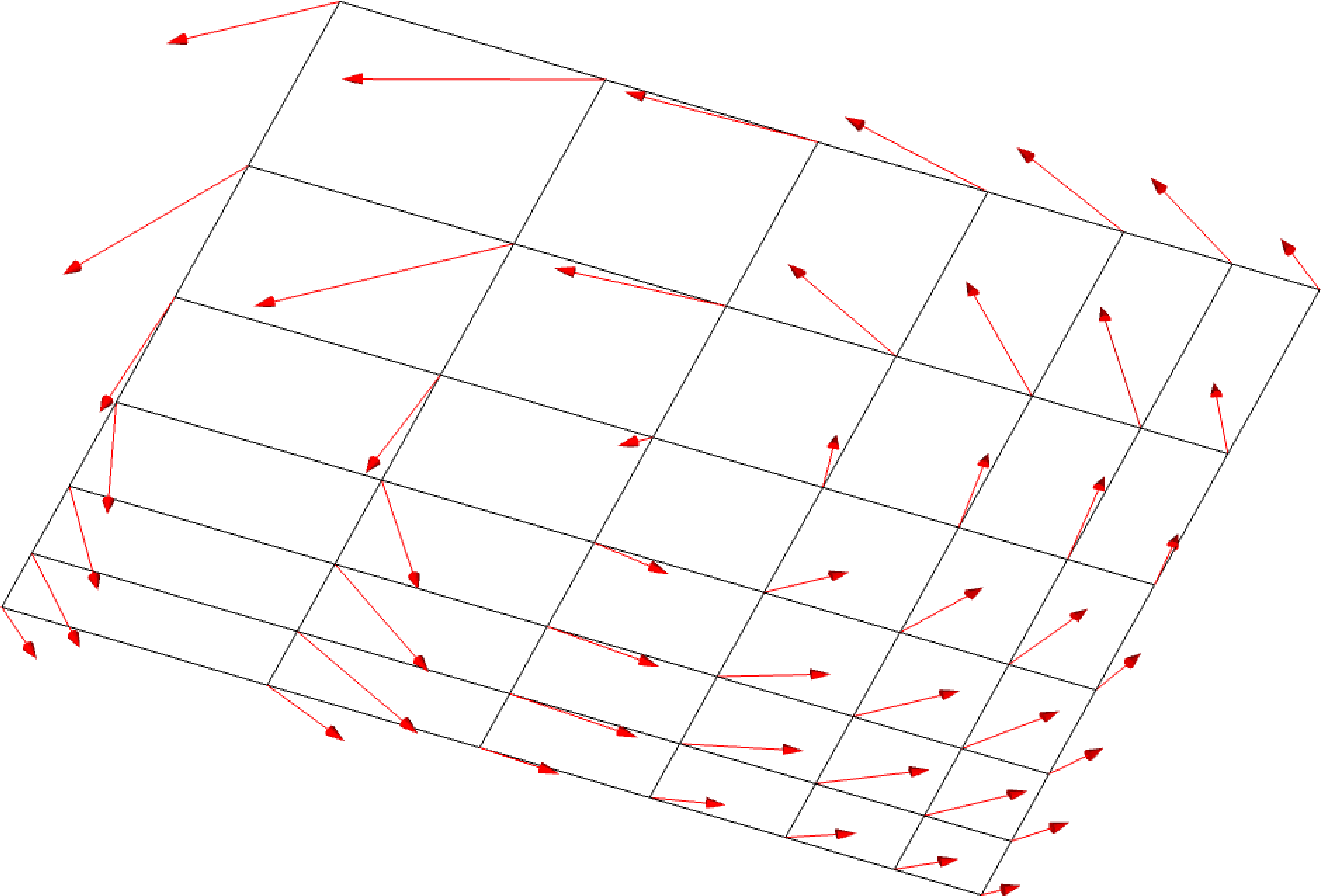
../../_images/mom_app.png — Fig. 7.5 Distributed Z moment load distribution.

7.8.5. Example: Applying Torque to Solid Bar

The following example for applying torque around an arbitrarily oriented shaft shown in Fig. 7.6. The coordinate system rod_1 is linked to nodes on the body and will update as the rod moves so that the torque is always applied around the rod axis.

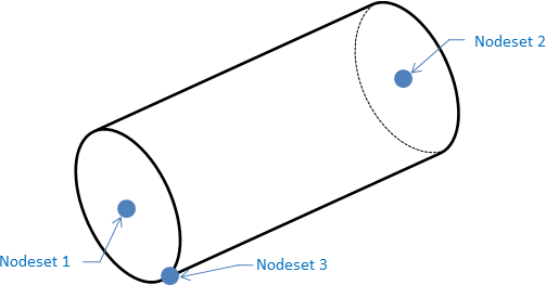
../../_images/DistLoadTorqueExample.png — Fig. 7.6 Distributed load example.

#  Define a body fitted coordinate system on the rod
begin rectangular coordinate system rod_1
  type   = rectangular
  # Base of Cylinder
  origin nodeset = nodelist_1
  # Vector from origin to vector nodes defines Z axis
  z point nodeset = nodelist_2
  # A point on the XY plane
  xz point nodeset = nodelist_3
end

#  Ramp up loading function
begin function ramp
  type is piecewise linear
   begin values
     0.00 0.0
     0.01 1.0
   end values
end

#  Apply a distributed load to the rod block, around the
#  axis of the cylindrical rod.
begin distributed moment
  block = block_1
  coordinate system = rod_1
  function = ramp
  # Z coordinate direction of coordinate system lies along
  # the rod axis
  component = z
end