5.1.2. Turbulent Flow Over A Cylinder
This tutorial shows how to set up a turbulent over cylinder in Fuego. This module has also been recorded in prior trainings and is available here or in the player below.
This is an extension of the previous tutorial Laminar Flow Over A Cylinder. If you have not completed that tutorial, please do so before starting this tutorial as the information discussed in the laminar flow tutorial will be used in this tutorial.
The governing equations employed by Fuego correctly capture the effects of turbulence, provided a fine enough mesh is used. However, in most cases, the finest mesh we can afford to use is not fine enough to resolve the turbulent fluctuations.
In those cases, a better prediction of the flow may be made by adding a turbulence model. For this training, we’re going to use the subgrid scale kinetic energy one-equation ( ) model.
For an in depth discussion on this model, please see Subgrid-Scale Kinetic Energy One-Equation LES Model.
) model.
For an in depth discussion on this model, please see Subgrid-Scale Kinetic Energy One-Equation LES Model.
5.1.2.1. Problem Files
The files required for this tutorial can be downloaded here, or found in a CEE environment at /projects/sierra100/TF/Fuego.
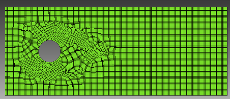
5.1.2.2. Problem Domain/Mesh
The problem domain and mesh are identical to the ones in Laminar Flow Over A Cylinder
5.1.2.3. Adding a Turbulence Model
5.1.2.3.1. Activating the Turbulent Kinetic Energy Equation
The first step is to activate the necessary equations and specify the turbulence model within Solution Options
The
model only requires the activation of the turbulent kinetic energy equationWe also need to add a block specifying the details of the turbulence model
Begin Solution Options
    Coordinate System = 2D
    Projection Method = Fourth_Order Smoothing with Timestep Scaling

    # DEFINE WHAT EQUATIONS TO SOLVE
    Activate Equation Continuity
    Activate Equation X_Momentum
    Activate Equation Y_Momentum
    Activate Equation turbulent_kinetic_energy

    # DEFINE NONLINEAR ITERATION SETTINGS
    Minimum Number of Nonlinear Iterations = 1
    Maximum Number of Nonlinear Iterations = 2

    # DEFINE ADVECTION SCHEME
    Upwind Method is MUSCL
    UPWIND LIMITER IS SuperBee

    Begin Turbulence Model Specification
        Turbulence Model = KSGS
    End

End   Solution Options
Here we activate the turbulent_kinetic_energy equation. This adds the turbulent kinetic energy (TKE) equation to the list of equations fuego will solve each time step. We must specify which
turbulence model to use, and in our case we will be using the KSGS model, which goes in the Turbulence Model Specification` block.
5.1.2.3.2. Applying Boundary Conditions and Initial Conditions
Begin Initial Condition Block FlowInit
    Volume is block_1
    Pressure   = 0.0
    X_Velocity = 0.0
    Y_Velocity = 0.0
    turbulent_kinetic_energy = 1e-4
End

# SET BOUNDARY CONDITIONS
Begin Inflow Boundary Condition on Surface surface_1
    X_Velocity = (2000*1.8e-5)/(1.2*0.1)
    Y_Velocity = 0.0
    turbulent_kinetic_energy = 1e-4
End

Begin Open Boundary Condition on Surface surface_2
    Pressure = 0.0
    turbulent_kinetic_energy = 1e-4
End

Begin Symmetry Boundary Condition on Surface surface_3
End

Begin Wall Boundary Condition on Surface surface_4
    post process yplus
End
The initial and boundary conditions for velocity and pressure are the same for the laminar tutorial, except now we must add conditions for the turbulent kinetic energy which is just a scalar degree of freedom.
Note that we did not add a boundary condition for TKE on the wall (surface_4) due to the fact that a zero-flux condition will be defaulted on the wall boundary. TKE must be a positive quantity, and cannot
go negative. If during the solution the TKE begins to go negative, Fuego will automatically “clip” the solution values to guarantee this to a lower limit determined by your problem units.
5.1.2.3.3. Results Output
Finally, we will add this new scalar DOF to our results output block
Begin Results Output Label Fuego_output
    Database Name = results/cylinder.e
    At Time 0, Interval = 0.1
    Title Turbulent backward facing step flow
    Nodal Variables = Pressure as P
    Nodal Variables = X_Velocity as Ux
    Nodal Variables = Y_Velocity as Uy
    Nodal Variables = yplus
    Nodal Variables = turbulent_kinetic_energy as TKE
End
5.1.2.4. Running Fuego and Reading The Logfile
To run Fuego, open a terminal and navigate to where your input files and mesh files are located, and run the following commands:
module load sierra
mpirun -n 4 fuego -i flow_over_cylinder_turb.i
Let’s take a quick look at the logfile to see what has changed from the laminar case
Step 2    , Time = 3.750e-03, dT = 2.250000e-03, Simulation is   0.0% complete

Fuego      Nonlinear Residuals of the Equation Sets     Linear    Linear
Nonlinear      Cell Reynolds number(max) =     168.6      Solver    Solver
Iteration              CFL(max) =    0.1636             Iterations Residual   DOF Min    DOF Max
--------- --------------------------------------------- ---------- --------  ---------- ----------
1 of  2 : SubMechanicsManager
1 of  1 :   MomentumSubMech
              X_Momentum                   = 7.05e-03      2      2.56e-13   7.01e-02   1.51e+00
              Y_Momentum                   = 6.89e-04      1      1.50e-07  -7.18e-01   7.05e-01
              Continuity                   = 1.45e-04      17     3.68e-09  -4.40e-01   8.72e-01
                Velocity pre-correction ----------------------------------->     0.07       1.51
                Velocity post-correction ---------------------------------->     0.01       0.60
1 of  1 :   KSGSSubMech
              Turbulent_Kinetic_Energy     = 1.99e-06      1      3.69e-08   9.87e-05   1.18e-02
  Fuego      Nonlinear Residuals of the Equation Sets     Linear    Linear
Nonlinear      Cell Reynolds number(max) =     168.6      Solver    Solver
Iteration              CFL(max) =    0.2455             Iterations Residual   DOF Min    DOF Max
--------- --------------------------------------------- ---------- --------  ---------- ----------
2 of  2 : SubMechanicsManager
1 of  1 :   MomentumSubMech
              X_Momentum                   = 4.80e-05      1      6.01e-08   1.16e-02   6.12e-01
              Y_Momentum                   = 1.77e-05      1      2.44e-07  -3.01e-01   2.97e-01
              Continuity                   = 4.66e-05      13     8.62e-09  -1.82e-01   4.50e-01
                Velocity pre-correction ----------------------------------->     0.01       0.61
                Velocity post-correction ---------------------------------->     0.01       0.61
1 of  1 :   KSGSSubMech
              Turbulent_Kinetic_Energy     = 2.42e-07      1      2.72e-08   9.87e-05   1.10e-02
Elapsed wall time = 0.60 seconds (0.21 s this step)
Notice that we are now tracking the Turbulent_Kinetic_Energy DOF in the logfile. It appears that the nonlinear residual is decreasing during the nonlinear iteration step, which is the expected behavior. This shows that
the TKE is converging. Again, always be checking the logfiles, they contain useful information about convergence rates and the DOF ranges.
5.1.2.5. Viewing Results
Please follow the steps from the previous tutorial to run ParaView Viewing Results.
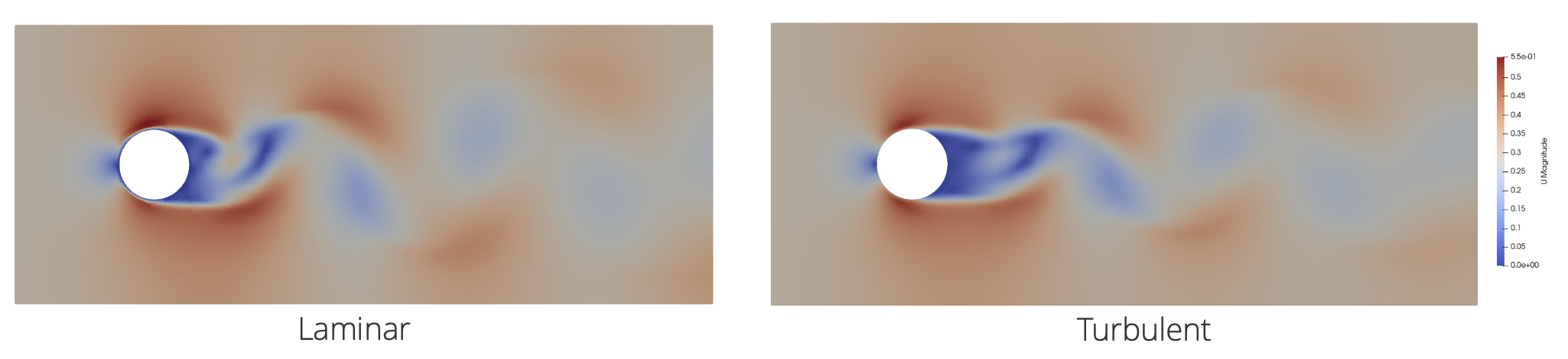
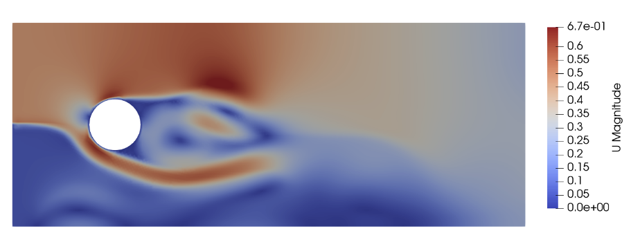
At what time does the flow break symmetry and start shedding? (Laminar was ~2 s) Does the wake structure look different? Does the boundary layer on the upstream side of the cylinder look different?
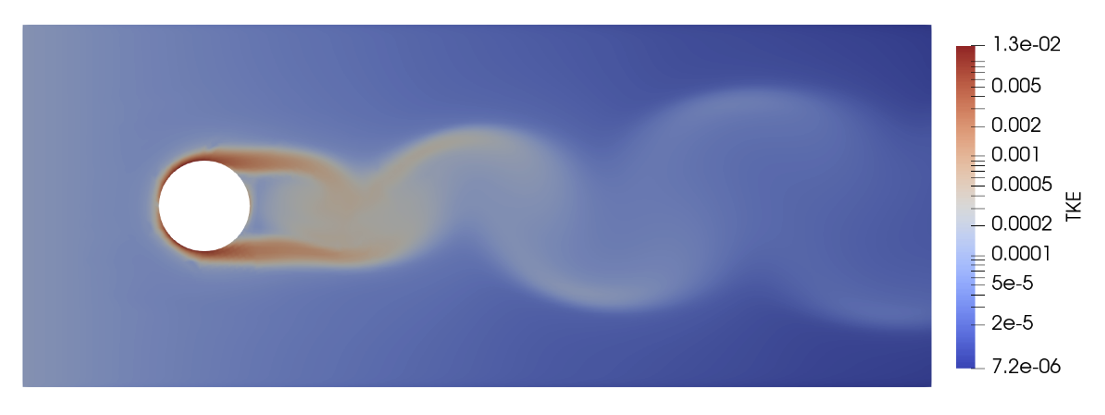
Look at the new TKE output field. Where is the turbulent kinetic energy highest?
5.1.2.6. Changing Boundary Conditions
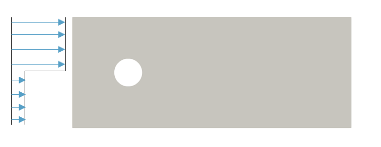
Let’s change the constant inflow condition to something more interesting
Begin Inflow Boundary Condition on Surface surface_1
  X_Velocity = "0.3*(1+0.75*sin(t)) * (y>0 ? 1 : 0.1)"
  Y_Velocity = 0.0
  Turbulent_Kinetic_Energy = 1.0e-4
End
Here, we replace the inflow boundary condition with a string function, illustrated in the image below
Run the code as usual, and visualize the results