5.1.3. Post-processing
This tutorial demonstrates some capabilities of the Fuego post-processor. This module has also been recorded in prior trainings and is available here or in the player below.
5.1.3.1. Problem Files
The files required for this tutorial can be downloaded here, or found in a CEE environment at /projects/sierra100/TF/Fuego.
5.1.3.2. Flux Post-processors
Flux post-processors are available in boundary condition blocks, e.g.
Begin Inflow Boundary Condition on Surface surface_1
    X_Velocity = (2000*1.8e-5)/(1.2*0.1)
    Y_Velocity = 0.0
    turbulent_kinetic_energy = 1e-4
    Postprocess total flux of continuity as mdot_in
End

Begin Open Boundary Condition on Surface surface_2
    Pressure = 0.0
    turbulent_kinetic_energy = 1e-4
    Postprocess total flux of continuity as mdot_out
End
Here we wish to postprocess the total mass flux in and out of the domain. For this, the general syntax is:
Postprocess [total|advective|diffusive] flux of [EQUATION] as [SOME_NAME]
In this particular case, two new global variables are created, mdot_in and mdot_out.
5.1.3.3. Post-processor Block
Scope: Region
Flux post-processors are available in boundary condition blocks, e.g.
Begin Postprocess point
    Output name = p_point
    Location = 0 0
    Function = "pressure"
End
In this example, we wish to postprocess the value of pressure at a specific point in space.

This will track the pressure over time at this specific point, with a global variable named p_point. Note that the function = "pressure" can be changed to another function. For instance, we can make a function that depends on
the x-velocity, or some other arbitrary function. This is shown in the integral post-processor in the next block
Begin Postprocess integral
    Output name = total_x_mom
    Location = all_blocks
    Function = "density * abs(x_velocity)"
End
In this case, the integral post-processor will spatially integrate the specified function over all blocks on the mesh.
For a list of other post-processor blocks see Postprocess.
5.1.3.4. Global Variable Output
5.1.3.4.1. Heartbeat Files
Heartbeat files are used in Fuego to track and output global variables, and print them in .csv files or plain text, column-formatted files.
Begin Heartbeat myHeartbeat
  Stream Name = heartbeat.csv
  Format = csv
  At Step 0 increment = 1
  Variable is Global time
  Variable is Global mdot_in
  Variable is Global mdot_out
  Variable is Global total_x_mom
  Variable is Global p_point as Pressure
End
In this example we have included all of the post-processed global variables from the previous sections. This block command will create a heartbeat file named heartbeat.csv in .csv format, and
will print out every time iteration in the Fuego run.
5.1.3.4.2. Results Output
Additionally we can track global variables in exodus output
Begin Results Output Label Fuego_output
  Database Name = results/cylinder.e
  At Time 0, Interval = 0.1
  Title Flow over a cylinder
  Nodal Variables = Pressure as P
  Nodal Variables = X_Velocity as Ux
  Nodal Variables = Y_Velocity as Uy
  Nodal Variables = yplus
  Global Variables = mdot_in
  Global Variables = mdot_out
  Global Variables = total_x_mom
  Global Variables = p_point
End
5.1.3.5. Running Fuego and Reading The Heartbeat File
To run Fuego, open a terminal and navigate to where your input files and mesh files are located, and run the following commands:
module load sierra
mpirun -n 4 fuego -i flow_over_cylinder_postproc.i
Let’s examine the heartbeat file
  time  ,      mdot_in,      mdot_out,    total_x_mom,   Pressure
0.00000e+00,  0.00000e+00,  0.00000e+00,  0.00000e+00,  0.00000e+00
1.50000e-03, -1.44000e-01,  1.44000e-01,  1.43907e-01,  1.19911e+02
3.75000e-03, -1.44000e-01,  1.44000e-01,  1.44103e-01,  2.36038e-04
7.12500e-03, -1.44000e-01,  1.44000e-01,  1.44069e-01,  5.50133e-04
1.21875e-02, -1.44000e-01,  1.44000e-01,  1.44024e-01,  5.55514e-04
1.97813e-02, -1.44000e-01,  1.44000e-01,  1.44002e-01,  5.55127e-04
3.11719e-02, -1.44000e-01,  1.44000e-01,  1.43996e-01,  5.53956e-04
All of our global variables are printed out in this heartbeat file. The heartbeat file can be visualized using your plotting software of choice (python, Excel, Matlab, even ParaView)
5.1.3.6. Viewing Results
Please follow the steps from the previous tutorial to run ParaView Viewing Results.
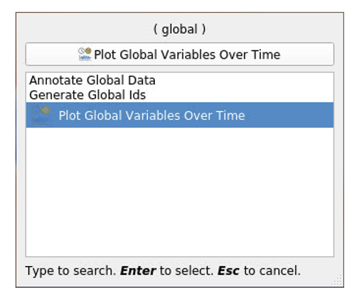
Once the solution is loaded into ParaView, navigate to the top menu Filters->Data Analysis->Plot Global Variables over Time.
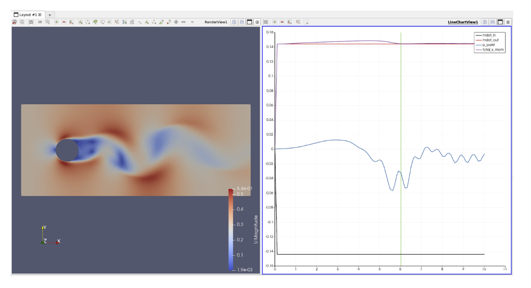
Color the results by velocity magnitude, and view the global variable data as a function of time