Sculpt

Sculpt is a separate parallel application designed to generate all-hex meshes on complex geometries with little or no user interaction. Sculpt was developed as a separate application so that it can be run independently from Cubit on high performance computing platforms. It was also designed as a separable software library so it can be easily integrated as an in-situ meshing solution within other codes. Cubit provides a front end command line and GUI for the Sculpt application. The command will build the appropriate input files based on the current geometry and can also automatically invoke Sculpt to generate the mesh and bring the mesh back to Cubit.

• Preparing to Use Sculpt
• Sculpt Parallel Command
• Sculpt Parallel Path Command
• Sculpt Examples
• Sculpt Technical Description
• Sculpt Application Documentation

Preparing to Use Sculpt

Platforms

Sculpt Installation

Sculpt is a stand-alone executable, separate from Cubit. In order for Cubit to start up Sculpt, it must be on your system and accessible to Cubit. The default installation of Cubit should install files in the correct locations for this to occur. Check with Cubit support if it did not come with your installation or you are not able to locate it or any of its supporting applications.

To run Sculpt from Cubit, four executable files are needed:

• sculpt: Application that controls start-up of mpiexec and psculpt. Main entry point from Cubit, that checks for the existence and compatibility of either the system mpiexec application or will use a local cubit instalation of mpiexec.
• psculpt: The main mpi-based Sculpt application. Requires mpiexec to run.
• mpiexec: Standard application available on most linux-based operating systems for starting up mpi-based applications on multiple processors. This should be available with your Cubit installation, but is also available from open-mpi.org
• epu: Used for combining multiple exodus files, generated with Sculpt, into a single exodus file. This executable is optional, but is useful for importing the resulting mesh into Cubit for viewing. It is part of the SEACAS tool suite developed by Sandia National Laboratories and is also included with your Cubit installation. It can also be obtained in open source form from sourceforge.net.

To view the current path to these executables that Cubit will use, issue the following command from the Cubit command window

 Sculpt Parallel Path List

See the Sculpt Parallel Path Command for more info on setting and customizing these paths.

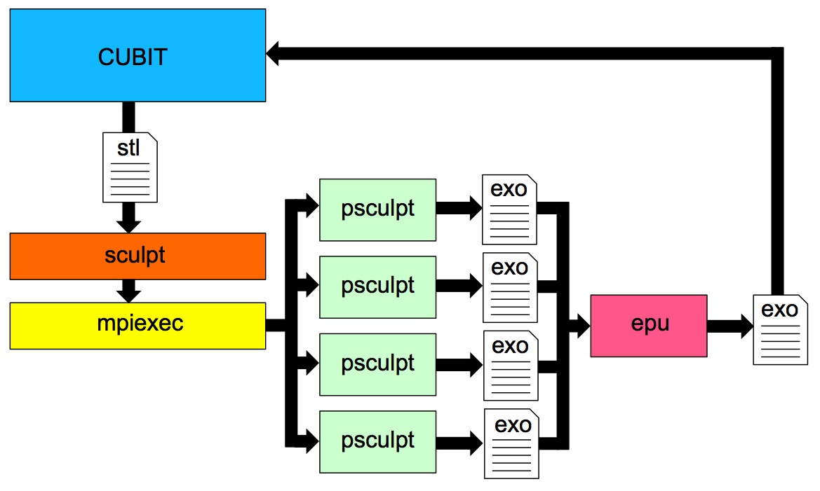
The following image illustrates the process flow when the sculpt parallel command is used in Cubit.

For the Sculpt meshing process, a set of files, including a facet-based stl file are written to disk. The sculpt application is then started up which in turn invokes mpiexec to start up multiple instances of psculpt in parallel. psculpt then performs the meshing and writes one exodus file per processor. These files can then be combined using epu and then imported back into Cubit for viewing.

Setting your Working Directory

When using the Sculpt Parallel command in Cubit, several temporary files will be written to the current working directory. Because of this, it is important to set your working directory before using Sculpt to a desired location where you want these files placed.

Sculpt Parallel Command

The command syntax for preparing a model for Sculpt is:

 Sculpt Parallel [Volume|Block <id_list>]
     [processors <value>]
     [fileroot '<root filename>']
     [exodus '<exodus filename>']
     [overwrite]
     [absolute_path]
     [no_execute]
     [size <value>|autosize <value>]
     [xint <value> yint <value> zint <value>]
     [box align|{Location <options> Location <options>}]
     [smooth <value>]
     [csmooth <value>]
     [num_laplace <value>]
     [max_opt_iters <value>]
     [opt_threshold <value>]
     [max_pcol_iters <value>]
     [pcol_threshold <value>]
     [max_deg_iters <value>]
     [deg_threshold <value>]
     [sideset <value>]
     [void]
     [stair <value>]
     [htet <value>]
     [pillow <value>]
     [adapt_type <value>]
     [adapt_threshold <value>]
     [adapt_levels <value>]
     [combine]
     [import]
     [show]
     [clean]
     [gen_input_file]

Sculpt Parallel Path Command

The command for letting Cubit know where the Sculpt and related applications are located is:

 Sculpt Parallel Path [List|Psculpt|Epu|Mpiexec]

Sculpt Mesh Quality Control

In most cases, the Sculpt tool can be used without adjusting default values. Depending on the characteristics of the geometry to be meshed, the default values may not yield adequate mesh quality. Upon completion, Sculpt reports to the command line, a summary of the mesh that was generated. This includes a summary of the mesh quality. Care should be taken to review this summary to ensure the minimum mesh quality is in a range suitable for analysis.

The element metric used for computing mesh quality in Sculpt is the Scaled Jacobian. This is a value between -1 and 1 that is a relative measure of the angles at the element's nodes. A value of 1 indicates a perfect 90 degree angle between each of its edges. In most cases a value less than zero, or negtive Jacobian element, indicates an unusable mesh. Sculpt's default settings try to achieve a minimum Scaled Jacobian of 0.2, which is normally usable in most analysis. The following discussion provides several options for adjusting the model or Sculpt parameters to help improve mesh quality.

1. Locating poor mesh quality: When the Sculpt mesh has been imported back into CUBIT it is a good idea to display the element quality. You can do this with variations of the following commands:

    quality hex all scaled jacobian
   quality hex all draw mesh
   

   Identify regions where hexes are poor quality and zoom in to these regions.
2. Modifying the geometry: Zooming in to poor quality elements may reveal that the mesh does not adequately represent the underlying geometry. In some cases you may find that small features, or small gaps between parts may be on the order of the size of the Sculpt cell size. If these features are not important to the analysis, you may consider using Cubit's geometry modification tools to remove features or close small gaps.
3. Modifying the cell size: In cases where small geometric features or gaps are important to the simulation, it may be necessary to use a smaller base cell size. Use the size or autosize input parameters or increase the numbers of intervals. Normally to adequately capture a feature you would want the cell size to be no greater than about 1/3 to 1/2 the size of the smallest feature you would want to represent in the simulation.
4. Turning on Pillowing for multiple materials: For models that have more than one material that share an interface, unless the geometry is precisely aligned with the global axis, it is usually a good idea to turn on pillowing. Pillowing automatically inserts an additional layer of hexes at interface boundaries to improve mesh quality. Without pillowing may notice inverted or poor quality elements at curve interfaces where 2 or more materials meet.
5. Modifying smoothing parameters: Sculpt includes a tiered approach to smoothing to improve element quality. It starts by applying smoothing to all nodes in the mesh and progressively restricts the smoothing operations to only those nodes that fall below a user-defined scaled Jacobian threshold. Default numbers of iterations and thresholds for each smoothing phase have been tuned for general use, however it may be worthwhile to adjust these parameters. The three smoothing phases include:
   • Laplacian Smoothing: Applied to all elements. Very inexpensive fast approach to improve quality, but can result in degraded element quality if applied to excess. A fixed default of 2 iterations is applied to all hexes. Increasing the num_laplace parameter can improve some cases, especially convex shapes
   • Optimization Smoothing: Applied only to elements who's scaled Jacobian falls below the opt_threshold parameter (default 0.6) and their surrounding elements. This approach uses a more expensive optimization technique to improve regions of elements simultaneously. The max_opt_iters parameter can control the maximum number of iterations applied (default is 5). Iterations will terminate, however, if no further improvement is detected. Because this method optimizes node locations simultaneously, neighboring nodes with competing optimum can sometimes limit mesh quality.
   • Spot Optimization: Also known as parallel coloring, is applied only to elements who's element quality falls below the pcol_threshold parameter (default 0.2). This technique is the most expensive of the techniques, but focusses only on nodes that are immediately adjacent to poor quality hexes. Each node is smoothed independently of its neighbors, and may require a high number of iterations using the max_pcol_iters to achieve desired results. Increasing the pcol_threshold and max_pcol_iters may yield improved results.
   Observing the mesh quality output to the command line following each smoothing iteration can provide some insight on the effect of modifying smoothing parameters.
6. Creating degenerate hexes: Some geometries will not permit a usable mesh with a traditional all-hex mesh. Sculpt includes the option to automatically and selectively collapse element edges to improve low-quality elements. The max_deg_iters and the deg_threshold values are used to control the creation of degenerates. Degenerate elements are treated as standard hex elements, but use repeated nodes in the eight-node connectivity array.
7. Creating hex-dominant mesh Another option for avoiding mesh quality issues is to generate a few tet elements in the mesh using the htet option. With this option you can specify a scaled Jacobian threshold value below which hexes will be converted to tet elements. The interface between hex and tet elements is managed by an automatically defined set of nodesets and sidesets that describe where multi-point constraints will be applied.

Sculpt Examples

• Basic Sculpt
• Size and Bounding Box
• Meshing the Void
• Automatic Sideset Definition
• Running Sculpt Stand-Alone
• Meshing Multiple Materials With Sculpt

The following examples use this simple geometry. Execute these commands prior to performing the example Sculpt Parallel command line operations

 sphere rad 1
sphere rad 1
vol 2 mov x 2
cylinder rad 1 height 2
vol 3 rota 90 about y
vol 3 mov x 1
unite vol all

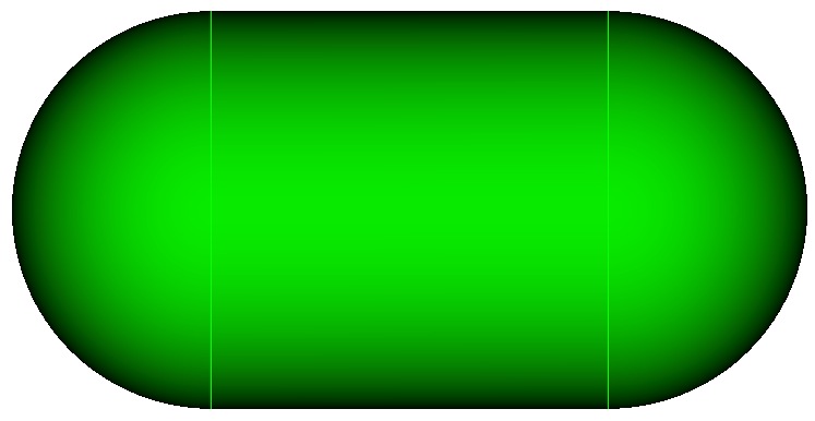
Figure 1. Geometry created from the above commands and used for the following examples.

Basic Sculpt

This example illustrates use of Sculpt with all default options. So that we can view the result, we will also use the overwrite, combine and import options.

 sculpt parallel over combine import
draw block all

The result of this operation is shown in Figure 2. For this example, behind the scenes, Cubit built an input file for Sculpt, ran it on 4 processors, combined the resulting 4 meshes, and subsequently imported the resulting mesh into Cubit. Note that Volume 1 remains "unmeshed" and we have created a free mesh that is not associated with a volume. The result of any Sculpt command is always an unassociated free mesh.

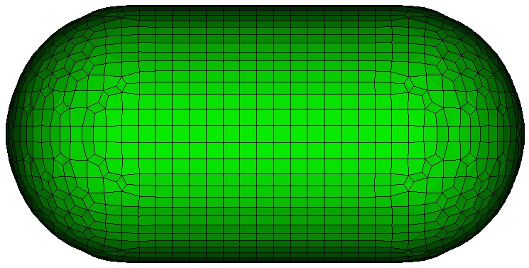
Figure 2. Free mesh generated from sculpt command

Size and Bounding Box

This example illustrates the use of the size and box options

 delete mesh
sculpt parallel size 0.1 box location position -1.5 0 -1.5 location position 1 1.5 0 over import combine
draw block all

In this case we have used the size option to define the base cell size for the grid. We have also used the box option to define a bounding box in which the mesh will be generated. Any geometry falling outside of the bounding box is ignored by Sculpt. Figure 3 shows the mesh generated with this command.

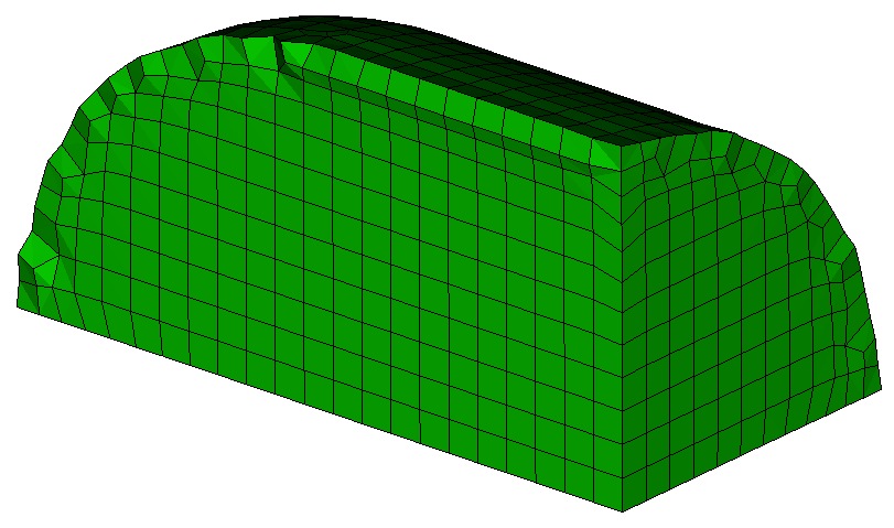
Figure 3. Sculpt "box" option limits the extent of the generated mesh.

Meshing the Void

In this example we illustrate the use of the void option:

 delete mesh
sculpt parallel size 0.1 box location position -1.5 0 -1.5 location position 1 1.5 0 over import combine void
draw block all

The result is shown in figure 4. Notice that this example is precisely the same as the last with the exception of the addition of the void option. Mesh is generated in the space surrounding the volume out to the extent of the bounding box. In this case, an additional material block is defined and automatically assigned an ID of 2. The nodes and element faces at the interface between the two blocks are shared between the two materials.

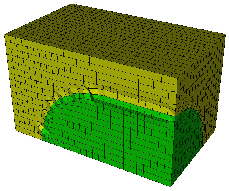
Figure 4. Sculpt "void" operation generates mesh outside the volume.

Automatic Sideset Definition

In this example we illustrate the use of the sideset option.

Generating sidesets on the free mesh with Cubit: Sideset boundary conditions can be manually created on the resulting free mesh from Sculpt using the standard Sideset <sideset_id> Face <id_range> syntax. The Group Seed command is also useful in grouping faces based on a feature angle to be used in a single sideset.

Generating sidesets in Sculpt: Sculpt also provides several options for defining sidesets as part of the Sculpt run. The following illustrates one option:

 delete mesh
sculpt parallel size 0.1 box location position -1.5 0 -1.5 location position 1 1.5 0 over import combine void sideset 2
list sideset all
draw sideset all

Once again we use the same syntax but add the sideset 2 option to automatically generate a series of sidesets. The list command should reveal that 10 sidesets were defined for this example with IDs 1 to 10. Figure 5 shows the result of the draw command showing all of the sidesets in different colors. Note that for the sideset 2 option, sidesets are created with the following criteria:

• Interfaces between materials
• Exterior surfaces
• Surfaces at the domain boundary

See the sideset option above for a description of other options for generating sidesets in Sculpt.

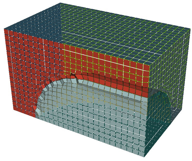
Figure 5. Automatic sidesets created using Sculpt

Running Sculpt Stand-Alone

Begin by setting your working directory to a location that is convenient for placing example files

 cd "path/to/my/sculpt/examples"

Next we issue the basic sculpt parallel command to mesh the volume

 delete mesh
sculpt parallel processors 8 fileroot "bean" over no_execute

In this case, we used the no_execute option which does not invoke the Sculpt application. Instead it will write a series of files to the working directory. The fileroot option defines the base file name for the files that will be written; in this case "bean". We also use the processors option to set the number of processors to be used to 8.

To see the files that Cubit placed in the working directory, bring up a terminal window on your desktop and change directories to the current working directory (ie. cd path/to/my/sculpt/examples). A directory listing should reveal 3 files as shown in Figure 6.

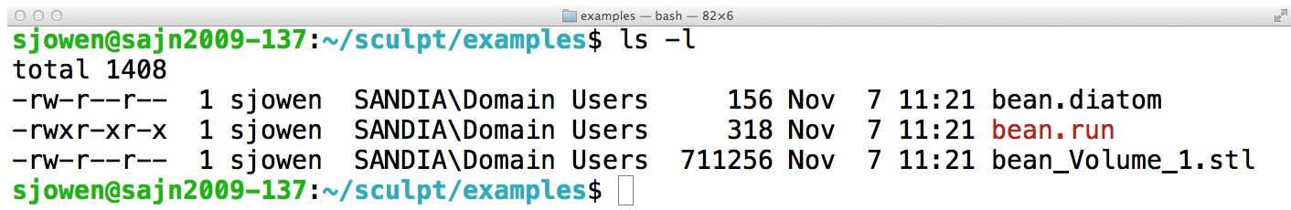
Figure 6. Directory listing of files written from Cubit

The following describes the purpose of each of the resulting files:

• bean.diatom: Diatoms is a file format used by Sandia's CTH and Alegra analysis programs that includes a rich constructive solid geometry definition. A series of directives for constructing and orienting primitives to build a complete solid model can be used. Included in the Diatom description is an STL import option. While any standard Diatom description may be used as input to Sculpt, for Cubit's purposes, only the STL option is used. This file contains a listing of all STL files that will be used as input to Sculpt.
• bean.run: The .run file contains the unix command line for running sculpt. Note that the file permissions have been set to execute to allow this file to be used as a unix script. Figure 7 shows the .run file for this example. Note that the command uses mpiexec and the psculpt executables, along with their full path. These paths may need to be edited when running on a different machine. It also includes the default parameters for setting the sizes, bounding box and smoothing parameters that have been computed by Cubit.

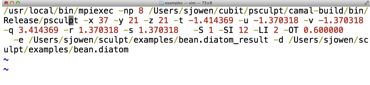
Figure 7. Unix command line for running Sculpt generated by Cubit

• bean_Volume_1.stl: The STL file is a copy of the geometric model. In our case, it is a representation of the cylinder and sphere object we have been working with. The STL format is a set of triangles that describe the surfaces of the object. One STL file will be generated for each Volume. If the Block option is used, then one file for each Block would be created.

To run sculpt on the same machine, from the terminal window in your current working directory you would issue the following command:

 ./bean.run

If Sculpt is to be run on a different machine, copy the files in the working directory to the other machine and issue the same command. Remember to change the path to the mpiexec and psculpt executables to match those on the new machine. For running on cluster machines that have scheduling of resources, check with your system administrator for how to submit a job for running.

After running Sculpt, Figure 8 shows the resulting files that would be written to the current working directory.

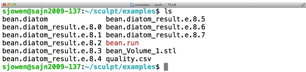
Figure 8. 8 Exodus files were generated and placed in working directory

Note that 8 exodus files have been generated, 1 from each processor. These files can be used by themselves or used as-is for use in a simlation, or they can be combined into a single file. The exodus files produced by Sculpt include all appropriate parallel communication information as defined by the Nemesis format. Nemesis is an extension of Sandia's Exodus II format that also includes appropriate parallel communication information.

To combine the resulting exodus files into a single file, we can use the epu tool. Epu should be included in your Cubit distribution, but may require you to set up appropriate paths for it to be recognized. To run epu on this model, use the following command from a unix terminal window:

 epu -p 8 bean.diatom_result

The result should be a single file with the name bean.diatom_result.e. The mesh in this file can then be imported into Cubit. Switch back to your Cubit application and from the command line type the following command:

 import mesh "bean.diatom_result.e" no_geom

The result should be the same mesh we generated previously that is shown in Figure 2.

Meshing Multiple Materials With Sculpt

 delete mesh
cylinder rad 0.5 height 3
cylinder rad 0.5 height 3
vol 5 mov x 2

The resulting geometry should look like the image in Figure 9.

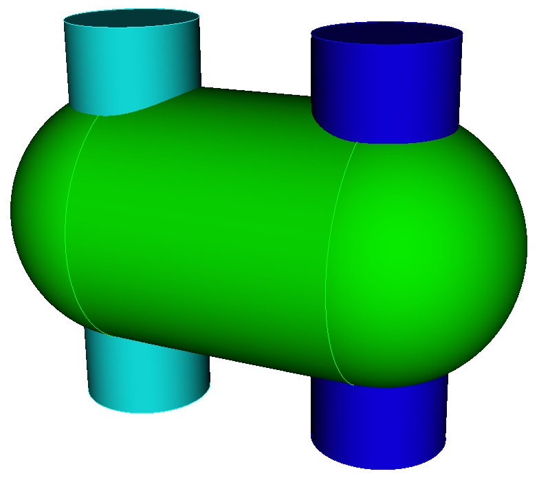
Figure 9. Geometry used to demonstrate multiple materials with Sculpt

Use this geometry to generate a mesh using Sculpt.

 sculpt parallel size 0.075 over combine import
draw block all

The resulting mesh should look like the image in Figure 10.

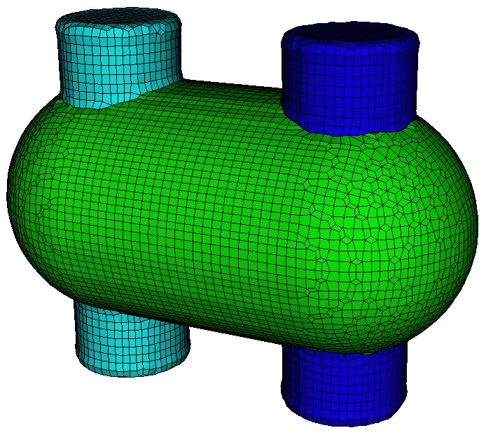
Figure 10. Mesh generated on multiple materials

Notice that one mesh block per volume was created. We should also note that no boolean operations were performed prior to building the mesh with Sculpt. In fact, volumes 4 and 5 were significantly overlapping volume 1. This would be an invalid condition for normal Cubit meshing operations. Figure 11 shows a cut-away image of the mesh using the Clipping Plane tool.

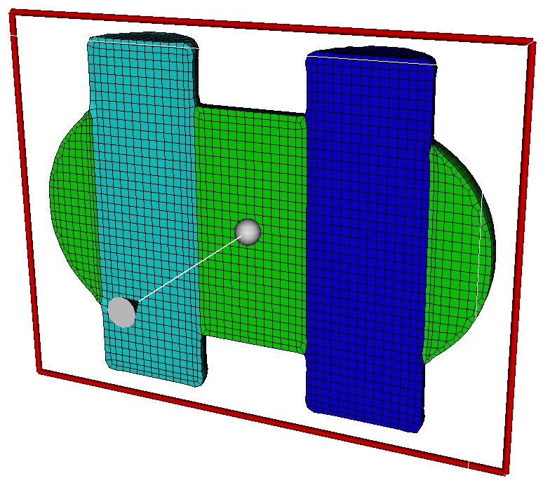
Figure 11. Cut-away of mesh generated on multiple materials

We should also note that imprint/merge operations typically needed, were also not required. While it is usually best to avoid overlaps to avoid ambiguities in the topology, Sculpt is able to generate a mesh giving precedence to the most recently defined materials. Merging is performed strictly by geometric proximity. Volumes closer than about one half the user input size will normally be automatically merged.

Next, we will examine the mesh quality of the free mesh. The following command will display a graphical representation of the Scaled Jacobian metric.

 quality hex all scaled jacobian draw mesh

The result is shown in Figure 12. Note the elements (colored red) at the interface between materials are unacceptable for simulation. This is caused by the Sculpt algorithm projecting nodes to a common curve interface shared by the materials.

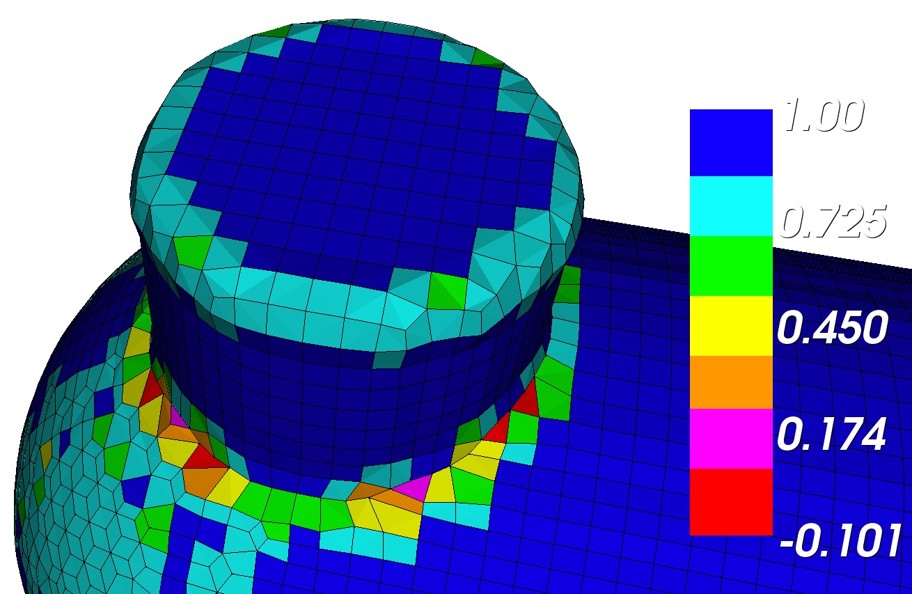
Figure 12. Mesh quality of multi-material mesh.

In most cases, the poor element quality at material interfaces can be improved by using the pillow option. Adding this option will direct Sculpt to add an additional layer of elements surrounding each surface. To see the result of pillowing, issue the following commands:

 delete mesh
sculpt parallel size 0.075 over combine import pillow 1
quality hex all scaled jacobian draw mesh

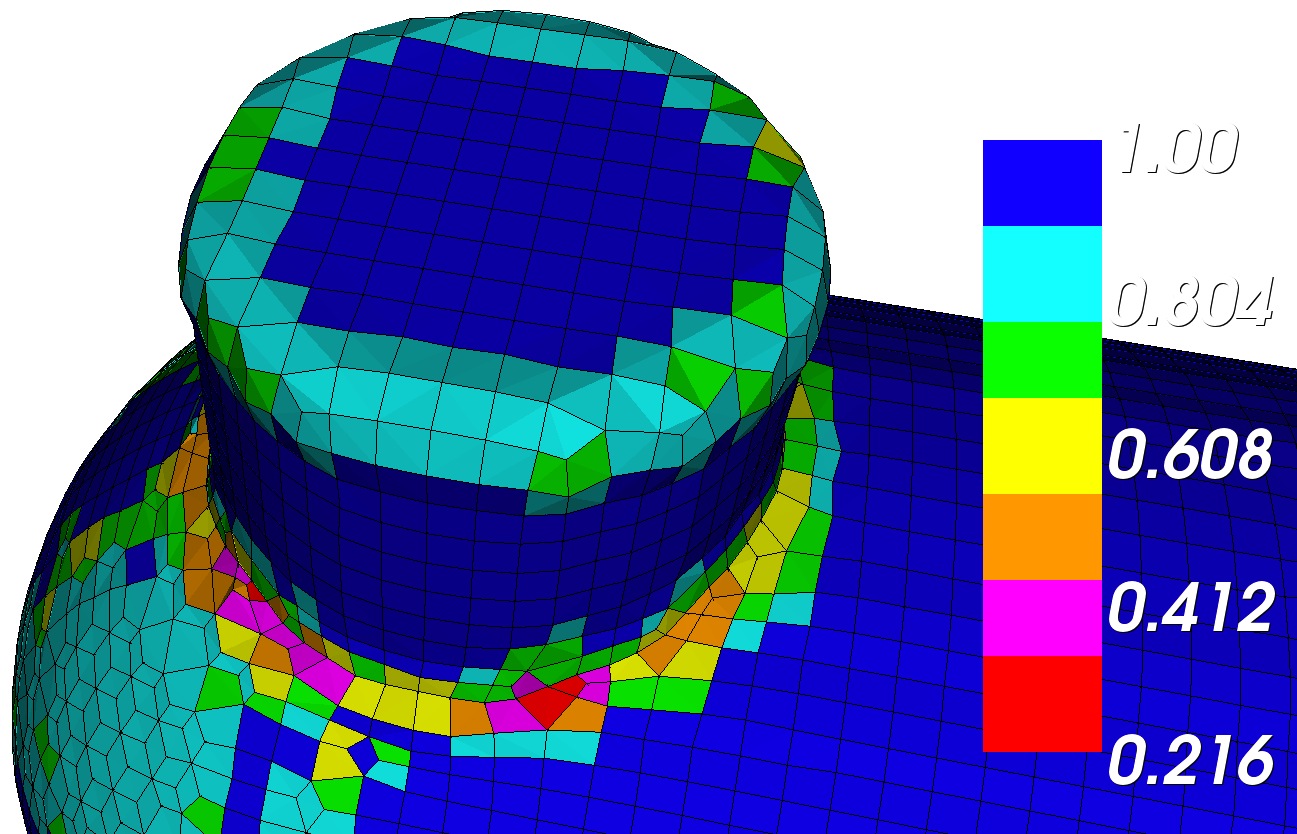
Figure 13. Mesh quality of multi-material mesh using pillow option

The resulting mesh is showed in Figure 13. Note the improved mesh quality at the shared curve interface. A closer look at the mesh, shown in Figure 14. reveals the additional layer of hexes surrounding each surface that allows for improved mesh quality when compared with Figure 11. When generating meshes with multiple materials that must share common interfaces, the pillow option is usually recommended.

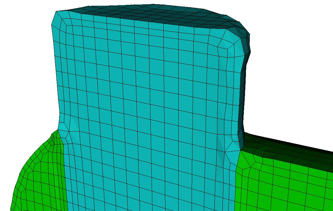
Figure 14. Cutaway of mesh reveals the additional layer of hexes surrounding each surface when the pillow option is used.