6.2. Element Sections

Element sections are defined by section command blocks. There are currently 11 different types of section command blocks. The section command blocks appear in the SIERRA scope, at the same level as the FINITE ELEMENT MODEL command block. In general, a section command block has the following form:

BEGIN section_type SECTION <string>section_name
  {command lines dependent on section type}
END [section_type SECTION <string>section_name]

Currently, section_type can be SOLID, COHESIVE, SHELL, MEMBRANE, BEAM, TRUSS, SPRING, DAMPER, POINT MASS, PARTICLE, or SUPERELEMENT. These various section types are identified as individual section command blocks and are described below. The corresponding section_name parameter in each of these command blocks, e.g., truss_section_name in the TRUSS SECTION command block, is selected by the user. The method used to associate these names with individual SECTION command lines in PARAMETERS FOR BLOCK command blocks is discussed in Section 6.1.7.5.

Following is a list of most of the different element formulations that are offered in Sierra/SM. The sections are colored bold, red, and blue based on where the documentation can be found. Bold sections do not have any documentation posted; prospective users should contact a developer before use. Red sections can be found in the Sierra/SM Capabilities in Development manual. Blue links to the relevant section in this manual.

Element	# nodes	Section	Formulation
ANY	ANY	RIGID BODY
ANY	ANY	SUPERELEMENT
Sphere	1	DEM
Sphere	1	PARTICLE	SPH
Sphere	1	PARTICLE	POINT MASS
BAR	2	BEAM
BAR	2	BOLT
BAR	2	CYLINDRICAL JOINT
BAR	2	DAMPER
BAR	2	LINEAR BEAM
BAR	2	SPRING
BAR	2	SPRING SUPPORT
BAR	2	TRUSS
BAR	2	USERMOUNT

Element	# nodes	Section	Formulation	Strain Incrementation
Shell	3	SHELL	ORIG_TRI_SHELL	MIDPOINT_INCREMENT
Shell	3	SHELL	ORIG_TRI_SHELL	STRONGLY_OBJECTIVE
Shell	3	SHELL	C0_TRI_SHELL	MIDPOINT_INCREMENT
Shell	3	SHELL	C0_TRI_SHELL	STRONGLY_OBJECTIVE
Shell	4	COHESIVE
Shell	4	MEMBRANE	MEAN_QUADRATURE	MIDPOINT_INCREMENT
Shell	4	MEMBRANE	MEAN_QUADRATURE	STRONGLY_OBJECTIVE
Shell	4	MEMBRANE	SELECTIVE_DEVIATORIC	MIDPOINT_INCREMENT
Shell	4	SHELL	NQUAD
Shell	4	SHELL	BT_SHELL	MIDPOINT_INCREMENT
Shell	4	SHELL	KH_SHELL	MIDPOINT_INCREMENT
Shell	4	SHELL	KH_SHELL	STRONGLY_OBJECTIVE
Shell	4	SHELL	BL_SHELL	MIDPOINT_INCREMENT
Shell	4	SHELL	BL_SHELL	STRONGLY_OBJECTIVE
TETRA		SOLID	MEAN_QUADRATURE	STRONGLY_OBJECTIVE
TETRA		SOLID	MEAN_QUADRATURE	NODE_BASED
TETRA		SOLID	FULLY_INTEGRATED	STRONGLY_OBJECTIVE
TETRA		SOLID	FULLY_INTEGRATED	NODE_BASED
TETRA		SOLID	VOID
PYRAMID	5	SOLID	MEAN_QUADRATURE	MIDPOINT_INCREMENT
PYRAMID	5	SOLID	MEAN_QUADRATURE	STRONGLY_OBJECTIVE
PYRAMID	5	SOLID	MEAN_QUADRATURE	TOTAL_LAGRANGE
WEDGE	6	COHESIVE
WEDGE	6	LOCAL
WEDGE	6	SOLID	MEAN_QUADRATURE	MIDPOINT_INCREMENT
WEDGE	6	SOLID	MEAN_QUADRATURE	STRONGLY_OBJECTIVE
WEDGE	6	SOLID	MEAN_QUADRATURE	TOTAL_LAGRANGE
HEX	8	COHESIVE
HEX	8	LOCAL
HEX	8	SOLID	FULLY_INTEGRATED
HEX	8	SOLID	MEAN_QUADRATURE	MIDPOINT_INCREMENT
HEX	8	SOLID	MEAN_QUADRATURE	STRONGLY_OBJECTIVE
HEX	8	SOLID	MEAN_QUADRATURE	TOTAL_LAGRANGE
HEX	8	SOLID	SELECTIVE_DEVIATORIC	STRONGLY_OBJECTIVE
HEX	8	SOLID	VOID
TETRA	8	NOT SUPPORTED
TETRA	10	SOLID	(NONE_SPECIFIED = COMPOSITE_TET)	STRONGLY_OBJECTIVE
TETRA	10	SOLID	FULLY_INTEGRATED
HEX	20	SOLID	FULLY_INTEGRATED	STRONGLY_OBJECTIVE
HEX	27	SOLID	FULLY_INTEGRATED	STRONGLY_OBJECTIVE

Table 6.2 TOTAL LAGRANGE SECTION

Element	# nodes	Formulation	Strain Incrementation	cubature
TETRA	4	FULLY_INTEGRATED	LOGARITHMIC_MAPPING	1
TETRA	4	FULLY_INTEGRATED	STRONGLY_OBJECTIVE	1
TETRA	4	FULLY_INTEGRATED	LOGARITHMIC_MAPPING	2
TETRA	4	FULLY_INTEGRATED	STRONGLY_OBJECTIVE	2
TETRA	4	FULLY_INTEGRATED	LOGARITHMIC_MAPPING	3
TETRA	4	FULLY_INTEGRATED	STRONGLY_OBJECTIVE	3
HEX	8	FULLY_INTEGRATED	LOGARITHMIC_MAPPING	ANY
HEX	8	FULLY_INTEGRATED	STRONGLY_OBJECTIVE	ANY
TETRA	10	COMPOSITE_TET	LOGARITHMIC_MAPPING	2
TETRA	10	COMPOSITE_TET	STRONGLY_OBJECTIVE	2
TETRA	10	FULLY_INTEGRATED	LOGARITHMIC_MAPPING	2
TETRA	10	FULLY_INTEGRATED	STRONGLY_OBJECTIVE	2
TETRA	10	FULLY_INTEGRATED	LOGARITHMIC_MAPPING	3
TETRA	10	FULLY_INTEGRATED	STRONGLY_OBJECTIVE	3
TETRA	10	FULLY_INTEGRATED	LOGARITHMIC_MAPPING	4
TETRA	10	FULLY_INTEGRATED	STRONGLY_OBJECTIVE	4
PYRAMID	13	FULLY_INTEGRATED	LOGARITHMIC_MAPPING	ANY
PYRAMID	13	FULLY_INTEGRATED	STRONGLY_OBJECTIVE	ANY
WEDGE	15	FULLY_INTEGRATED	LOGARITHMIC_MAPPING	ANY
WEDGE	15	FULLY_INTEGRATED	STRONGLY_OBJECTIVE	ANY
HEX	20	FULLY_INTEGRATED	LOGARITHMIC_MAPPING	ANY
HEX	20	FULLY_INTEGRATED	STRONGLY_OBJECTIVE	ANY
HEX	27	FULLY_INTEGRATED	LOGARITHMIC_MAPPING	3
HEX	27	FULLY_INTEGRATED	STRONGLY_OBJECTIVE	3
HEX	27	FULLY_INTEGRATED	LOGARITHMIC_MAPPING	5
HEX	27	FULLY_INTEGRATED	STRONGLY_OBJECTIVE	5

Table 6.3 Default section for solid elements

Solid Element Type	Section Type	Formulation	Strain Formulation
HEX8	SOLID	MEAN QUADRATURE	MIDPOINT INCREMENT
HEX20	SOLID	FULLY INTEGRATED	STRONGLY OBJECTIVE
HEX27	SOLID	FULLY INTEGRATED	STRONGLY OBJECTIVE
TET4	SOLID	MEAN QUADRATURE	STRONGLY OBJECTIVE
TET10	TOTAL LAGRANGE	COMPOSITE TET	STRONGLY OBJECTIVE
WEDGE6	SOLID	MEAN QUADRATURE	MIDPOINT INCREMENT
PYRAMID5	SOLID	MEAN QUADRATURE	MIDPOINT INCREMENT

6.2.1. Solid Section

BEGIN SOLID SECTION <string>solid_section_name
  RVE COORDINATE SYSTEM = <string>Coordinate_system_name
  FORMULATION = <string>MEAN_QUADRATURE|SELECTIVE_DEVIATORIC|
    FULLY_INTEGRATED|VOID(MEAN_QUADRATURE)
  DEVIATORIC PARAMETER = <real>deviatoric_param
  STRAIN INCREMENTATION = <string>MIDPOINT_INCREMENT|
    STRONGLY_OBJECTIVE|NODE_BASED|TOTAL_LAGRANGE(depends)
  STRESS MEASURE = CAUCHY|HENCKY(CAUCHY)
  NODE BASED ALPHA FACTOR = <real>bulk_stress_weight(0.01)
  NODE BASED BETA FACTOR = <real>shear stress_weight(0.35)
  NODE BASED STABILIZATION METHOD = <string>EFFECTIVE_MODULI|
    MATERIAL(MATERIAL)
  HOURGLASS FORMULATION = <string>TOTAL|INCREMENTAL|
    HYPERELASTIC(INCREMENTAL)
  HOURGLASS INCREMENT = <string>ENDSTEP|MIDSTEP (ENDSTEP)
  HOURGLASS ROTATION = <string> APPROXIMATE|SCALED (APPROXIMATE)
  RIGID BODY = <string>rigid_body_name
  RIGID BODIES FROM ATTRIBUTES = <integer>first_id
    TO <integer>last_id
  MASS LUMPING METHOD = DEFAULT|ROWSUM|EVEN (DEFAULT)
END [SOLID SECTION <string>solid_section_name]

The SOLID SECTION command block specifies the properties for solid elements (hexahedra and tetrahedra). This command block is to be referenced by an element block made up of solid elements. The two types of solid-element topologies currently supported are hexahedra and tetrahedra. The parameter solid_section_name is user-defined and is referenced by a SECTION command line in a PARAMETERS FOR BLOCK command block.

The RVE COORDINATE SYSTEM command line specifies the name of a coordinate system definition block command used to define a local coordinate system on each element of a block that uses this SOLID SECTION. This coordinate system only has an effect on RVE analysis (see the Sierra/SM Capabilities in Development manual for details).

The FORMULATION command line specifies whether the element will use a single-point integration rule (mean quadrature), a selective-deviatoric rule, a selectively integrated rule, or a fully-integrated rule, or act as a void element. The selective-deviatoric and fully-integrated integration rules are higher-order integration schemes, which are discussed below.

If the user wishes to use the selective-deviatoric rule, the DEVIATORIC PARAMETER command line must also appear in the SOLID SECTION command block.

Choosing the SELECTIVE_DEVIATORIC formulation indicates that the element is fully integrated with respect to the deviatoric stress response and under integrated with respect to the hydrostatic pressure response. The under-integration of the hydrostatic pressure response is achieved through averaging the pressure over the integration points. The SELECTIVE_DEVIATORIC formulation is often used to alleviate volumetric locking associated with isochoric motion. By default, this formulation involves no hourglass control. However, the user may include an additional input command within the element section, DEVIATORIC PARAMETER, which may set deviatoric_param between 0.0 and 1.0, and which blends an under-integrated deviatoric stress field (DEVIATORIC PARAMETER = 0.0) with a fully-integrated deviatoric stress field (DEVIATORIC PARAMETER = 1.0). Setting a value of 0.0 results in an under-integrated element type without any hourglass control, and is not recommended. By default, this parameter is set to 1.0, which is the recommended value in almost all circumstances. Lower values, ideally not less than 0.5, may improve convergence or accuracy in some very specific circumstances.

The selective-deviatoric elements, when used with a value greater than 0.0, provide hourglass control without artificial hourglass parameters.

Alternatively, a fully-integrated rule can be defined by setting FORMULATION = FULLY_INTEGRATED. This will apply an eight-point integration scheme for eight-noded hexahedral elements and a four-point integration scheme for ten-noded tetrahedral elements. This definition is currently unavailable for four-noded and eight-noded tetrahedral elements.

The VOID formulation is valid for 8-node hexahedral and 4-node tetrahedral element blocks. Void elements only compute volume. They do not contribute internal forces to the model. The material model and density associated with void elements are ignored. The volume and the first and second derivatives of the volume for each element are stored in the element variables volume, volume_first_derivative, and volume_second_derivative. The volume derivatives are computed using least squares fits of the volume history, which is stored for the previous five time steps.

In addition to the per-element volume and derivatives, the total volume and derivatives of that total volume for all elements in each void element block are written to the results file as global variables. The names for these variables are voidvol_blockID, voidvol_first_deriv_blockID, and voidvol_second_deriv_blockID. In these global variable names, blockID is the ID of the block. For example, the void volume for block 8 would be stored in voidvol_8.

The STRAIN INCREMENTATION command defines the strain incrementation formulation to use for solid element types that support multiple formulations. The element summary at the beginning of Section 6.1 specifies the strain incrementation formulations available for each element. Many elements have two choices for the strain incrementation formulation: MIDPOINT_INCREMENT or STRONGLY_OBJECTIVE. Generally, the midpoint-increment formulation is slightly faster and the strongly-objective formulation is slightly more accurate. Consult [[1], [2]] for descriptions of these strain formulations.

The four-noded tetrahedron has a NODE_BASED option for the STRAIN INCREMENTATION, which indicates usage of the node-based tetrahedron (see Section 6.2.1.1).

The eight-noded mean-quadrature hexahedron has a TOTAL_LAGRANGE option for the STRAIN INCREMENTATION, which is based on the total deformation and is provided for usage with the HYPERELASTIC hourglass formulation.

The STRESS MEASURE option is specifically for the eight-noded mean-quadrature hexahedron with the TOTAL_LAGRANGE strain incrementation and the HYPERELASTIC hourglass formulation. The HENCKY option is slightly more accurate for the hyperelastic hourglass formulation, but CAUCHY (the default) is necessary for optimal compatibility with the material models.

The HOURGLASS FORMULATION command is used to switch between total, hyperelastic and incremental forms of hourglass control. The total hourglass option can only be used with eight-noded mean-quadrature hexahedral elements using strongly objective strain incrementation (STRAIN INCREMENTATION = STRONGLY_OBJECTIVE). In contrast, the hyperelastic hourglass option can only be used with eight-node mean-quadrature hexahedral elements using total-Lagrange strain incrementation (STRAIN INCREMENTATION = TOTAL_LAGRANGE). One of the following three arguments can be used with this command: TOTAL, HYPERELASTIC, or INCREMENTAL.

The total formulation performs stiffness hourglass force updates based on the rotation tensor from the polar decomposition of the total deformation gradient. The hyperelastic formulation computes hourglass strains relative to the reference/model configuration, and has a well defined hyperelastic hourglass strain energy; as a result this formulation results in a symmetric contribution to the stiffness matrix, is fully reversible, and allows for a nonlinear hourglass resistance. The incremental formulation is the default and performs stiffness hourglass force updates based on the hourglass velocities and the incremental rotation tensor. The viscous hourglass forces and the hourglass parameters are unchanged by this command. Consult the element documentation [[2]] for a description of the hourglass forces and the incremental hourglass formulation.

The HOURGLASS INCREMENT and HOURGLASS ROTATION commands control the speed and accuracy of the hourglass control computation. These commands are only applicable to the mean-quadrature hexahedron with midpoint strain incrementation ({STRAIN INCREMENTATION = MIDPOINT_INCREMENT). The HOURGLASS INCREMENT line command specifies whether the hourglass resistance increment is to be computed at the middle or end of the time step. The end-step calculation has a slightly reduced computational cost while the mid-step computation is more accurate. The default is ENDSTEP. The HOURGLASS ROTATION command controls whether the hourglass resistance will be scaled after rotation to preserve the magnitude. Scaling requires additional computation time but will be more accurate, particularly when large rotations are present in the analysis. The default is APPROXIMATE, meaning no scaling is done.

Rigid elements in a section are indicated by including the RIGID BODY command line. The RIGID BODY command line specifies an identifier that maps to a rigid body command block. See Section 6.3.1 for a full discussion of how to create rigid bodies and Section 6.3.1.1 for information on the use of the RIGID BODIES FROM ATTRIBUTES command.

Known Issue

For problems with large rotations the hourglass energies are known to spike exponentially with increases in total rotation. This may be due to a coupling with hypoelastic material models.

6.2.1.1. Node-Based Tetrahedra

The node-based formulation can only be used with four node tetrahedral elements. If the element-block (i.e., PARAMETERS FOR BLOCK) command block has a SECTION command line that references a SOLID SECTION command block that uses

STRAIN INCREMENTATION = NODE_BASED

then the tetrahedral element block will use the node-based tetrahedron formulation.

The node-based formulation calculates a solution that is a mixture of an element-based formulation (information from the center of an element) and a node-based formulation (information at a node that is based on the average of all elements attached to the node). The node-based tetrahedron allows a model with four-node tetrahedral elements to avoid most of the locking problems of regular tetrahedral elements. Regular tetrahedral elements are much too stiff and can produce inaccurate results in many situations.

The mixture of node-based versus element-based information incorporated into the solution may be adjusted with the NODE BASED ALPHA FACTOR and NODE BASED BETA FACTOR command lines. These two lines apply only if the NODE_BASED option is specified on the STRAIN INCREMENTATION command line. The value for bulk_stress_weight on the NODE BASED ALPHA FACTOR command line sets the element bulk stress weighting factor, while the value for shear_stress_weight on the NODE BASED BETA FACTOR command line sets the element shear stress weighting factor. The weighting factors are described in detail in [[3]]. A strictly node-based formulation results when both factors are set to zero, while a strictly element-based formulation results when both factors are one.

The mixing of node-based and element-based solutions for the node-based formulation is a stabilization technique to eliminate zero energy modes of a pure node-based formulation. With this in mind, two options are provided for the stress update of the element-based solution through the NODE BASED STABILIZATION METHOD command (applicable only with STRAIN INCREMENTATION = NODE_BASED). The default option, MATERIAL, runs the same material model in the element as is run at the nodes, with independent material states. The other option, EFFECTIVE_MODULI, uses a linearized update for the element stress state based on the element average value of the nodal effective moduli. The nodal effective moduli are computed from the nodal stress and strain increments at each time step. This second option avoids potential issues due to having independent node and element material states.

Node based elements store material state, stress, and strain data at the nodes in addition to at the element center. Most element based quantities such as stress have similarly named nodal equivalents.

If a node is attached to only elements of one material type that node will have one set of state, stress and strain data that is the average of the attached element quantities.

If elements of multiple materials are attached to the same node then that node will store multiple independent sets of state variables. To accommodate this the node based state data is given a unique name by appending a unique index number to the end of each state variable name.

The log file contains a table that defines the mapping from the index number the nodal element block. For example:

========NODAL BASED TETRAHEDRA ELEMENT BLOCK AND MATERIAL INFORMATION ==========

   Block    Nodal State Index
  -------   -----------------
  block_1     1
  block_7     2
  block_200   3

================================================================================

Block 1, 7, and 200 are using nodal based tetrahedra element formulation. The nodal based stress in block 7 would be found in the nodal state variable stress_2. If a node was on a block boundary and attached to elements of block block 1 and block 7 then that node would have both stress_1, the stress associated with the block 1 material, and stress_2, the stress associated with the block 7 material. Note that for nodal based tetrahedra these nodal stresses and material states are the most relevant quantities to visualize. Additionally note that many derived output quantities such as the von Mises stress norm are not hooked to the nodal based output quantities.

The MASS LUMPING METHOD is used to set the algorithm for determination of the lumped nodal masses. The ROWSUM option means first compute the consistent mass matrix then set the lumped mass of each node as the sum of the consistent mass matrix row. The ROWSUM method gives more accurate gravity loads and a more consistently stable explicit time step. Row sum is the default method for most elements. The EVEN option means take the total element mass and divide it evenly between the elements nodes. The EVEN method exists mostly to allow backwards compatibility with previous Sierra/SM versions where the even mass lumping method was always used. The DEFAULT method means the code automatically picks the best mass lumping option based on element type. For most elements this is the row sum method. A few elements perform better with even mass lumping and use this method as the default.

Note that there also exist other solid element formulations which can be specified in the separate TOTAL LAGRANGE section block. These options are currently documented in the in development manual.

6.2.1.2. 10-Node Tetrahedron Default Formulation

The MEAN_QUADRATURE formulation has been deprecated for 10-node tetrahedron elements for robustness and accuracy reasons. The default formulation for the 10-node tetrahedron is the COMPOSITE_TET. This element can be used by creating an empty solid section, by not specifying a section in the block definition, or by using a Total Lagrange section. The default values for the COMPOSITE_TET are VOLUME AVERAGE J = ON and STRAIN_INCREMENTATION = STRONGLY_OBJECTIVE. See section Section 6.2.2 for more details.

6.2.2. Total Lagrange Section

Total Lagrangian [[4]] formulations are written in terms of Lagrangian measures of stress and strain, where derivatives are taken with respect to the Lagrangian or material coordinates. This differs from the approach used in most other element formulations in the code including the uniform gradient hex, which computes derivatives with respect to the Eulerian or spatial coordinates. The currently implemented finite element topologies for the total Lagrange section are the 8-noded hexahedron, 20-noded hexahedron, 27-noded hexahedron, 13-noded pyramid, 4-noded tetrahedron, 10-noded tetrahedron, and 15-noded wedge.

BEGIN TOTAL LAGRANGE SECTION <string>section_name
  FORMULATION = <string>{FULLY_INTEGRATED|
    COMPOSITE_TET}(FULLY_INTEGRATED)
  STRAIN INCREMENTATION = <string>{STRONGLY_OBJECTIVE|
    LOGARITHMIC_MAPPING}(STRONGLY_OBJECTIVE)
  CUBATURE DEGREE = <integer>degree
  VOLUME AVERAGE J = <string>{ON|OFF}

  # VEM stabilization for tet10 elements
  VEM STABILIZATION PARAMETER = <real>vem_shear_penalty(0.1)
  VEM BULK STABILIZATION PARAMETER = <real>vem_bulk_penalty(1.0e-6)
  VEM EXPONENT = <real>vem_exponent(5.0)
END [TOTAL LAGRANGE SECTION <string>section_name]

6.2.2.1. Formulation

FORMULATION = <string>{FULLY_INTEGRATED|
  COMPOSITE_TET}(FULLY_INTEGRATED)

The FORMULATION command defaults to the FULLY_INTEGRATED formulation for the given finite element topology.

For the 10-noded tetrahedral topology, the COMPOSITE_TET option exists, which uses a piecewise linear nodal basis instead of the standard quadratic nodal basis. As stated in Reference [[5]], the element is classified as composite because conceptually it consists of 12 sub-elements, each of which is a linear, 4-noded tetrahedron. Thus, the basis functions used to represent nodal fields are piecewise linear within the element. The deformation gradient and stress fields are assumed to live in a linear space, and the resulting gradient operator incorporates the projection of the piecewise discontinuous gradients into the assumed linear basis. The current implementation does not restrict the mid-edge nodes to be co-linear with the vertex nodes, allowing for better geometric resolution for curved bodies.

6.2.2.2. Strain Incrementation

STRAIN INCREMENTATION = <string>{STRONGLY_OBJECTIVE|
  LOGARITHMIC_MAPPING}(STRONGLY_OBJECTIVE)

In the total Lagrange formulation, the deformation gradient is always calculated as the derivative of the current configuration with respect to the reference configuration,

\[\mathbf{F}_{n+1}=\frac{\partial\mathbf{x}_{n+1}}{\partial\mathbf{X}}.\]

It follows that the incremental deformation gradient is defined as the deformation gradient between the configurations at times \(n\) and \(n+1\) and can be written in terms of \(\mathbf{F}_{n}\) and \(\mathbf{F}_{n+1}\),

\[\mathbf{f}_{n+1}=\mathbf{F}_{n+1}\mathbf{F}_{n}^{-1}.\]

The STRAIN INCREMENTATION command is then specific to hypoelastic material models, that is, models that use the rate of deformation to increment the stress. Two approaches are available: the STRONGLY_OBJECTIVE option in the context of the total Lagrange formulation mirrors what is found in the SOLID_SECTION as described in [[1]],

\[\mathbf{d}_{n+1}=\frac{1}{2\Delta t}\mathrm{log}\left(\mathbf{f}_{n+1}\mathbf{f}_{n+1}^{\scriptstyle{T}}\right);\]

the LOGARITHMIC_MAPPING option is computationally more expensive, but comparatively more accurate in problems with large rotations,

\[\mathbf{d}_{n+1}=\mathrm{sym} \frac{1}{\Delta t}\mathrm{log}\left(\mathbf{f}_{n+1}\right)\]

6.2.2.3. Cubature Degree

CUBATURE DEGREE = <integer>degree

This option effectively determines the number of integration points to be employed during numerical integration. For hexahedral elements, CUBATURE DEGREE = 3 corresponds to 8 integration points, and for tetrahedral elements, CUBATURE DEGREE = 3 corresponds to 5 integration points. The default is CUBATURE DEGREE = 5 for the FULLY_INTEGRATED 27-noded hexahedron and CUBATURE DEGREE = 3 for all other FULLY_INTEGRATED formulation elements (note the COMPOSITE_TET formulation described below is fixed at CUBATURE DEGREE = 2 and may not be changed with this option).

The following topology, formulation, and cubature combinations are available:

ELEMENT FAMILY	NUM. NODES	FORMULATION	CUBATURE DEGREE(S)
hexahedron	8	fully_integrated	3
	20	fully_integrated	3
	27	fully_integrated	5
pyramid	13	fully_integrated	3
tetrahedron	4	fully_integrated	1, 2, 3
	10	fully_integrated	2, 3, 4
tetrahedron	10	composite_tet	2
wedge	15	fully_integrated	3

6.2.2.4. Volume Average J

VOLUME AVERAGE J = <string>{ON|OFF}

This command is used to construct a deformation gradient where the dilatational component is volume-averaged over the element domain. It is applicable for implicit and explicit problems employing nearly incompressible material response, such as metal plasticity, and may provide less stiff solutions in that case. In addition, if this command is ON, then the hydrostatic component of the stress is also volume averaged. The default setting is OFF for the FULLY_INTEGRATED formulation and ON for the COMPOSITE_TET formulation.

6.2.2.5. VEM Stabilization for 10-noded Tetrahedral Elements

VEM STABILIZATION PARAMETER = <real>vem_shear_penalty(0.1)
VEM BULK STABILIZATION PARAMETER = <real>vem_bulk_penalty(1.0e-6)
VEM EXPONENT = <real>vem_exponent(5.0)

The VOLUME AVERAGE J = ON option avoids pressure modes but sacrifices the coercivity of the system, which may lead to displacement instabilities. A stabilization inspired by the virtual element method [[6]] (VEM) is provided to suppress the displacement modes with the options VEM STABILIZATION PARAMETER = <real>vem_shear_penalty, VEM BULK STABILIZATION PARAMETER = <real>vem_bulk_penalty, and VEM EXPONENT = <real>vem_exponent. VEM STABILIZATION PARAMETER and VEM BULK STABILIZATION PARAMETER act like hourglass stiffnesses scaled by the shear and bulk moduli, respectively, and the VEM EXPONENT controls how quickly the stabilization stiffens under large dilitation within the element. These VEM command options are only activated for fully-integrated and composite tet10 elements with CUBATURE DEGREE = 2 and VOLUME AVERAGE J = ON. The defaults are generally recommended but the optimal values can be problem dependent, so each can be set at the user’s discretion.

6.2.3. Cohesive Section

BEGIN COHESIVE SECTION <string>cohesive_section_name
  FORMULATION = <string>FULLY_INTEGRATED|UNDER_INTEGRATED(FULLY_INTEGRATED)
  LAYER THICKNESS = <real>layer_thickness(0.0)
END [COHESIVE SECTION <string>cohesive_section_name]

Warning

In order for the cohesive elements to contribute to the global stable time step, a node based time step must be used. See Section 3.2.3 for details.

The COHESIVE SECTION command block specifies the properties for cohesive zone elements (quadrilateral and triangular). The name of this block (given by cohesive_section_name) is referenced by the element block for cohesive elements. If the option for adaptive insertion of cohesive zone elements is used, the name of this block is referenced by the COHESIVE SECTION command defined in Section 6.5.7.

FORMULATION specifies the number of integration points for the cohesive element. The default is to fully integrate the element, which means the larger of the two possible number of integration points is used. It should be noted that with a single integration point (or under-integrating the element in general), spurious hourglass-like modes may be introduced to the deformation of the cohesive element. Therefore it is recommended to keep the default full integration schemes. Currently, the quadrilateral cohesive element supports either one or four integration points, the triangular cohesive element supports either one or three integration points, and the composite triangular cohesive element supports either four or twelve integration points.

The LAYER THICKNESS specifies the thickness to use for determining the mass of the cohesive element layer. A cohesive element is formulated as a surface element which implies that there is no volume to the element. Specifying a layer thickness allows the cohesive element to remain a surface element but have mass. This option is especially useful for cohesive elements that are meshed independently and tied to the remaining mesh with MPCs. Mass is required for motion to occur in dynamics. The element wise mass element_mass will be the cse_initial_area multiplied by the LAYER_THICKNESS and the DENSITY specified in the cohesive material model.

Warning

LAYER_THICKNESS is not supported with shell and wedge cohesive elements.

6.2.4. Localization Section

BEGIN LOCALIZATION SECTION <string>localization_section_name
  MEAN DILATATION FORMULATION
  NUMBER OF INTEGRATION POINTS = <integer>num_int_points
  THICKNESS = <real>thickness
  MEMBRANE FORCES = ON | OFF (ON)
END [LOCALIZATION SECTION <string>localization_section_name]

Warning

Currently the localization elements do not contribute to the global stable time step. As such, the user must specify a time step via the INITIAL TIME STEP and TIME STEP INCREASE FACTOR command lines. See Section 3.1 for details.

6.2.4.1. Kinematics

Localization elements [[7]] are planar elements that lie between bulk (volumetric) elements and can employ the same underlying bulk material model. Topologically, localization elements are identical to cohesive surface elements. The reason this 2D surface element can access 3D material models is due to the multiplicative decomposition of the deformation gradient \(\mathbf{F}\) such that \(\mathbf{F} = \mathbf{F}^{\parallel} \mathbf{F}^{\perp}\). Each portion of the decomposition can be expressed as

(6.1)\[{\mathbf{F}}^{\perp} = {\mathbf{I}} + \frac{\lbrack\!\lbrack \mathbf{\varPhi}\rbrack\!\rbrack}{h} \otimes {\mathbf{N}}, \qquad {\mathbf{F}}^{\parallel} = \mathbf{g}_{i} \otimes \hat{\mathbf{G}}^{i}\]

where \(\mathbf{F}^{\parallel}\) encapsulates in-plane stretching and \(\mathbf{F}^{\perp}\) reflects the displacement jump \(\lbrack\!\lbrack \mathbf{\varPhi} \rbrack\!\rbrack\) in the intermediate configuration which can be pushed to the current configuration through \(\lbrack\!\lbrack \mathbf{\varphi} \rbrack\!\rbrack = \mathbf{F}^{\parallel} \lbrack\!\lbrack \mathbf{\varPhi} \rbrack\!\rbrack\). Fig. 6.2 illustrates the kinematic construction.

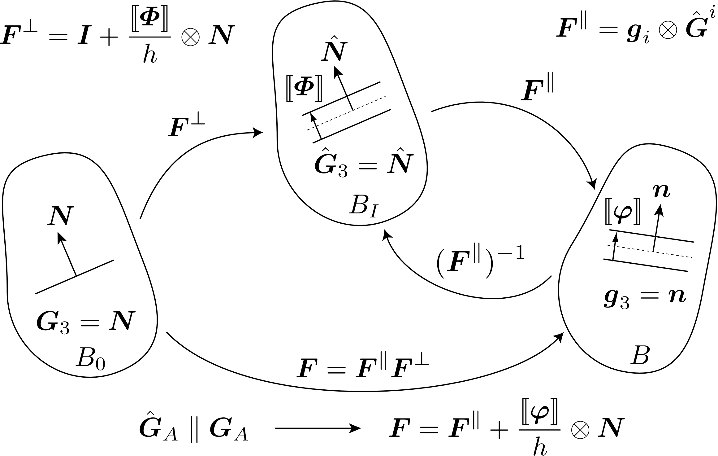
Fig. 6.2 The reference \(B_{0}\), intermediate \(B_{I}\), and current configuration \(B\) of the body. By redefining the jump in the intermediate configuration, the formulation simplifies to an additive decomposition having contributions from membrane stretching and the jump.

The jump is normalized by \(h\) which one can envision as an element thickness or a characteristic length scale governing separation. Quantities are considered to be constant through the thickness \(h\). The curvilinear basis vectors in the reference and current configuration are \(\mathbf{G}_{A}\) and \(\mathbf{g}_{i}\), respectively. Given that \(\mathbf{N}\) is constructed to be normal to the in-plane basis vectors \(\mathbf{G}_{A}\) in the reference configuration, one can prove that the in-plane basis vectors in the intermediate configuration are equivalent to the in-plane basis vectors in the reference configuration (\(\hat{\mathbf{G}}_{A} = \mathbf{F}^{\perp} \mathbf{G}_{A} = \mathbf{G}_{A}\)). One can then express the multiplicative decomposition as an additive decomposition thus simplifying the initial formulation given in [[7]].

(6.2)\[{\mathbf{F}} = {\mathbf{F}}^{\parallel} + \frac{\lbrack\!\lbrack \mathbf{\varphi} \rbrack\!\rbrack}{h} \otimes {\mathbf{N}}\]

Because the length scale \(h\) is independent of the discretization, the methodology is regularized and ideal for employing a local, softening material model to simulate the failure process. Details concerning the force calculation are available in [[7]].

6.2.4.2. Command summary

The LOCALIZATION SECTION command block specifies the properties for localization elements (quadrilateral and triangular). The name of this block (given by localization_section_name) is referenced by the element block for localization elements.

MEAN DILATATION FORMULATION

This command line will yield a constant pressure formulation. The average pressure is obtained at all integration points through a modification of the kinematic quantities. For hypo-elastic materials, \(\text{tr}[\mathbf{D}]\) is volume-averaged. For uncoupled hyperelastic models, \(\text{det}[\mathbf{F}]\) is volume-averaged. After volume averaging \(\text{tr}[\mathbf{D}]\) and \(\text{det}[\mathbf{F}]\), local dilatational contributions are removed, and additively (hypoelastic) or multiplicatively (hyperelastic) include the volume-averaged response. This results in an average pressure (by construction) and has been shown to be effective in avoiding element locking during isochoric deformations. Note that one can use a single integration point to achieve a constant pressure, but hourglass control is not provided to suppress spurious modes. If isochoric deformations are of concern, it is recommended to use a fully-integrated element with the MEAN DILATATION FORMULATION. The MEAN DILATATION FORMULATION will only be applied if the command is given in the LOCALIZATION SECTION.

NUMBER OF INTEGRATION POINTS = <integer>num_int_points

The default number of integration points for a localization element depends on the topology, but is always sufficient for full integration. For an eight-noded hexahedron (planar four-noded quadrilateral) the default is four integration points while for a six-noded wedge (planar three-noded triangle) the default is one integration point. However, it should be noted that with a single integration point, spurious hourglass modes can be introduced into the deformation of the quadrilateral localization element. Currently, the quadrilateral localization element supports one and four integration points while the triangular localization element supports one integration point.

THICKNESS = <real>thickness

The THICKNESS command line sets the localization element thickness \(h\). In many respects, \(h\) should be considered a material parameter as it governs the evolution of surface separation. The introduction of \(h\) generates the true length scale in the problem: the process zone size. Care must be taken to adequately resolve the process zone size or the methodology will not be regularized.

MEMBRANE FORCES = ON | OFF (ON)

The MEMBRANE FORCES command line should be used when the element size \(l\) is on the order of \(h\). In this specific case, the membrane forces will be sufficiently large to corrupt the crack-tip fields. If \(h \sim l\), we recommend that the membrane forces be OFF. Turning off membrane forces alters the force calculation to only employ the referential traction \(\mathbf{T} = \mathbf{P}\mathbf{N}\). In this sense, the formulation becomes “cohesive.” But because \(\mathbf{F}^{\parallel}\) is still employed in the kinematics to capture critical quantities such as the triaxiality, the stiffness matrix is no longer symmetric; however, the residual is correct. Numerous studies in implicit quasi-statics and implicit dynamics have confirmed that CG is still robust. To avoid non-monotonic reductions in the residual, one might employ solvers that can handle non-symmetric systems (ML) and solution methods other than CG (Newton with a line search) to obtain improved rates of convergence.

Warning

Domain decomposition may generate domains in which localization elements are isolated. Neither the upper or lower surface is connected to a bulk element. Because the localization element does contain a zero-energy membrane mode that is suppressed through bulk element assembly, the user will receive warnings that indicate additional rigid body modes on particular processors. To remedy the issue, the user can employ tangent diagonal scaling in the preconditioner. Studies have show this solution to be effective with minimal impact on the rate of convergence.

6.2.4.3. Usage guidelines

In contrast to cohesive surface elements, localization elements can employ bulk constitutive models for surface separation. For a typical application, the analyst might

• Identify a constitutive model that captures the failure process. This might include a local damage model or any model that employs strain softening to facilitate strain localization.

• Conduct mesh-dependent simulations with bulk elements of size \(s\) to understand potential paths for crack initiation and growth in specimen geometries targeted for parameterizing constitutive model parameters.

• Seed potential paths in specimen geometries and incorporate \(h\) into the fitting process. The fitting process may not be unique in that the same far-field response might be obtained from multiple combinations of both \(h\) and the material parameters that govern the failure process. An initial guess to being the iterative process might include \(h = 1/4 s\). Ensure that for all cases of \(h\) that the process zone that evolves is resolved.

• Consider the possibility of only enabling strain softening in the constitutive model that drives surface separation. Although this will assure that localization will occur in the surface elements, regulating softening to the seeded plane can introduce non-smoothness in the failure process.

• Understand the impact of \(h\). If \(h\) is too large, the fields governing the failure process will be less smooth and the additional compliance can create additional nonlinearities that can complicate implicit solution. Please consider refitting model parameters with lower values of \(h\). If \(h\) is too small, the localization element thickness will drive the condition number of the implicit system.

• Explore component or system level geometries with seeded paths for crack initiation and propagation. Additional simulations with bulk elements may be conducted to highlight potential failure paths. Refine the mesh to ensure that the far-field predictions are indeed mesh independent and that the process zone that evolves from the given micromechanics regularized by the length scale \(h\) is resolved.

• Inspect of the process zone with a focus on the local metrics that drive the failure process. For example, if stress triaxiality drives void growth, one should examine fields of triaxiality in both the bulk and localization elements. In contrast to other methods like the \(J\)-integral that focus on a driving force evaluated at some radius from the crack tip, localization elements seek to capture the resistance at the crack tip. Consequently, crack-tip fields must be resolved.

• Reflect on the fields employed for model parameterization and the fields evolving in component and system level models. If possible, align field evolution in component/system geometries with field evolution in specimen geometries. Disparities may drive the need for additional calibration experiments.

Although these usage guidelines have not focused on incorporating stochastic processes, one may sample distributions in material parameters. The inclusion of a method for regularization enables such findings in that the mesh-dependence associated with fracture/failure is not convoluted with a stochastic representation of the micro-mechanical process.

6.2.5. Shell Section

BEGIN SHELL SECTION <string>shell_section_name
  THICKNESS = <real>shell_thickness
  THICKNESS MESH VARIABLE =
    <string>THICKNESS|<string>var_name
  THICKNESS TIME STEP = <real>time_value
  THICKNESS SCALE FACTOR = <real>thick_scale_factor(1.0)
  CONTACT THICKNESS SCALE FACTOR = <real>thick_scale_factor(thick_scale_factor)
  INTEGRATION RULE = TRAPEZOID|GAUSS|LOBATTO|SIMPSONS|
    USER|ANALYTIC|CODE_SELECTED(CODE_SELECTED)
  NUMBER OF INTEGRATION POINTS = <integer>num_int_points(5)
  FORMULATION = KH_SHELL|BT_SHELL|BL_SHELL|NQUAD|
    C0_TRI_SHELL|ORIG_TRI_SHELL (BT_SHELL"QUAD" or ORIG_TRI_SHELL"Tri")
  RIGID BODY PROJECTOR =
    NONE|DRILLING_ONLY|ROTATIONS_AND_DRILLING (ROTATIONS_AND_DRILLING)
  BEGIN USER INTEGRATION RULE
    <real>location_1 <real>weight_1
    <real>location_2 <real>weight_2
    .
    .
    <real>location_n <real>weight_n
  END [USER INTEGRATION RULE]
  LOFTING FACTOR = <real>lofting_factor(0.5)
  LOFTING FACTOR MESH VARIABLE = <string>var_name
  OFFSET MESH VARIABLE = <string>var_name
  ORIENTATION = <string>orientation_name
  DRILLING STIFFNESS FACTOR = <real>stiffness_factor(1.0e-5)
  RIGID BODY = <string>rigid_body_name
  RIGID BODIES FROM ATTRIBUTES = <integer>first_id
    TO <integer>last_id
  STABLE TIME STEP ESTIMATE = COURANT|GERSCHGORIN(GERSCHGORIN)    

  CONTACT THICKNESS = <real>contactThickness
  CONTACT LOFTING FACTOR = <real>contactLofting

  FIBER ORIENTATION = <real>angle(0)
  R VECTOR READ VARIABLE = <string>rVecName
  T VECTOR READ VARIABLE = <string>tVecName
END [SHELL SECTION <string>shell_section_name]

The SHELL SECTION command block specifies the properties for a shell element. If this command block is referenced in an element block of three-dimensional, four-node elements, the elements in the block will be treated as shell elements. The parameter, shell_section_name, is user-defined and is referenced by a SECTION command line in a PARAMETERS FOR BLOCK command block.

Either a THICKNESS command line or a THICKNESS MESH VARIABLE command line must appear in the SHELL SECTION command block.

If a shell element block references a SHELL SECTION command block with the command line:

THICKNESS = <real>shell_thickness

then the thickness of all shell elements in the block will be initialized to the value shell_thickness.

Sierra/SM can also initialize the thickness using an attribute defined on elements in the mesh file. Meshing programs such as PATRAN and Cubit typically set the element thickness as an attribute on the elements. If the elements have one and only one attribute defined on the mesh, the THICKNESS MESH VARIABLE command line should be specified as

THICKNESS MESH VARIABLE = THICKNESS

which causes the thickness of the element to be initialized to the value of the attribute for that element. If there are zero attributes or more than one attribute, the thickness variable will not be automatically defined, and the command will fail.

The thickness may also be initialized by a scalar element field on the input mesh. To specify a field other than the single-element attribute, use the following form of the THICKNESS MESH VARIABLE command line:

THICKNESS MESH VARIABLE = <string>var_name

Here, the string var_name is the name of the initializing element field.

The input mesh may have values defined at more than one point in time. To choose the point in time in the mesh file that the variable should be read, use the command line

THICKNESS TIME STEP = <real>time_value

The default time point in the mesh file at which the variable is read is 0.0.

Once the thickness of a shell element is initialized by using either the THICKNESS command line or the THICKNESS MESH VARIABLE command line, this initial thickness value can then be scaled using the scale-factor command line:

THICKNESS SCALE FACTOR = <real>thick_scale_factor

If the initial thickness of the shell is 0.15 inch, and the value for thick_scale_factor is 0.5, then the scaled thickness of the membrane will be 0.075.

The thickness mesh variable specification may be coupled with the THICKNESS SCALE FACTOR command line. In this case, the thickness mesh variable is scaled by the specified factor.

CONTACT THICKNESS SCALE FACTOR = <real>contact_thick_scale_factor

The CONTACT THICKNESS SCALE FACTOR command is used for overwriting the value of THICKNESS SCALE FACTOR for contact purposes.

If the initial thickness of the shell is 0.15 inch, the value of thick_scale_factor is 0.5, and the value of contact_thick_scale_factor is 1.0, then the shell contact thickness will be equal to the original thickness (0.15) inches.

The thickness mesh variable specification may be coupled with the CONTACT THICKNESS SCALE FACTOR command line. In this case, the thickness mesh variable is scaled by the specified factor for contact.

The shell formulation can be selected via the FORMULATION command line. Several options are available:

• The BT_SHELL option is used to select the Belytschko-Tsay (BT) shell formulation. This is the default. The BT shell formulation has constant transverse shear, and is the fastest shell element available. Note, this element can experience stability issues at large in-plane strains.

• The BL_SHELL option is used to select the Belytschko-Leviathan (BL) shell formulation. The BL shell element is similar to the Belytschko-Tsay element but has additional shear terms and hourglass controls that the BT does not have. It also includes a projection of the angular velocities and the internal forces. The BL can better solve problems with high gradients of transverse shear (such as twisted beams), and no hourglass control or drilling stiffness is needed. Note, this element can experience stability issues at large in-plane strains.

• The KH_SHELL option specifies the Key-Hoff shell formulation, which includes a nonlinear transverse shear term. The Key-Hoff shell can better solve problems with high gradients of transverse shear (such as twisted beams), but distorted (non-rectangular) elements can be excessively stiff. Note, this element can experience stability issues at large in-plane strains.

• The NQUAD option selects a formulation for a completely elastic plate.

• The C0_TRI_SHELL option specifies the triangular shell formulation developed by Kennedy, Belytschko, and Lin (1986). The \(C^{0}\) tri shell is a robust, versatile element that uses an incremental strain computation, making it applicable to large strains. Note that this element has no resistance to rotations about the axis perpendicular to its plane.

• The TRI_SHELL option is a specialized triangular shell formulation. The option is in development and generally should not be used in production runs.

For the Belytschko-Leviathan shell formulation (BL_SHELL), the user may specify which rigid body modes to project out of the local velocity and force vectors via the RIGID BODY PROJECTOR command. The options are NONE, DRILLING_ONLY, and ROTATIONS_AND_DRILLING (the default). The NONE option indicates no rigid body modes are projected out and is only recommended for explicit analyses with relatively flat geometry. The DRILLING_ONLY option removes modes associated with the drilling degrees of freedom which are unconstrained in the 5-DoF family of shell elements. The ROTATIONS_AND_DRILLING option is a full projection that removes rigid body rotations and the drilling modes and is appropriate if warped shells are present. The last option also preserves angular momentum but leads to a stiffer response for the BL shell [[8], [9]].

Warning

The RIGID BODY PROJECTOR command is currently only available for the Belytschko-Leviathan shell formulation. The use of this command with other shell formulations has no effect.

For shell elements, the user may select from a number of integration rules, including a user-defined integration option. The integration rule is selected with the command line

INTEGRATION RULE = <string>TRAPEZOID|GAUSS|LOBATTO|SIMPSONS|
  ANALYTIC|CODE_SELECTED|USER(CODE_SELECTED)

Consult the element documentation [[2]] for a description of different integration schemes for shell elements.

For most material models the code will by default select the five point TRAPEZOID through the thickness integration rule. The code selected integration scheme for the elastic material model is ANALYTIC, which is an analytic through-thickness integration scheme. This scheme is significantly faster and slightly more accurate than any of the point-wise rules but only valid for fully elastic shell formulations.

Currently the analytic integration scheme is only available for the elastic material model when using the BT_SHELL and BL_SHELL shell formulations for quad shell elements.

Shells using the analytic integration rule do not compute integration point material or stress quantities such as stress, strain, or the various quantities derived from stress and strain. If integration point quantities are desired for elastic material shells, the shells can be forced to use a point-wise integration scheme by manually setting the integration rule to TRAPEZOID or another point-wise rule.

For all integration schemes, the through-thickness integration points are indexed starting at the point closest to the bottom surface with respect to the positive normal direction (See Fig. 6.3). For example, when requesting unrotated_stress_xx for a shell element using 5 integration points through the thickness, unrotated_stress_xx_1 corresponds to the integration point closest to the bottom surface and unrotated_stress_xx_5 corresponds to the integration point closest to the top surface.

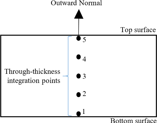
Fig. 6.3 Indexing convention for through-thickness integration points.

The number of integration points for the piecewise integration point rules can be set to any number greater than one by using the following command line:

NUMBER OF INTEGRATION POINTS = <integer>num_int_points(5)

The SIMPSONS, GAUSS, and LOBATTO integration schemes in the INTEGRATION RULE command line all default to five integration points. The number of integration points for these three schemes can be reset by using the NUMBER OF INTEGRATION POINTS command line. There are limitations on the number of integration points for some of these integration rules. The SIMPSONS rule can be set to any number greater than one, the GAUSS scheme can be set to one through seven integration points, and the LOBATTO integration scheme can be set to two through seven integration points.

In addition to these standard integration schemes, the USER INTEGRATION RULE command block may be used to define a custom integration scheme.

BEGIN USER INTEGRATION RULE
  <real>location_1 <real>weight_1
  <real>location_2 <real>weight_2
  .
  .
  <real>location_n <real>weight_n
END [USER INTEGRATION RULE]

A standard integration scheme and a user scheme may not be specified simultaneously. If the USER option is specified in the INTEGRATION RULE command line, a set of integration locations with associated weight factors must be specified. This is done with tabular input command lines inside the USER INTEGRATION RULE command block. The number of command lines inside this command block should match the number of integration points specified in the NUMBER OF INTEGRATION POINTS command line. For example, to use a user-defined scheme with three integration points, the NUMBER OF INTEGRATION POINTS command line should specify three (3) integration points and the number of command lines inside the USER INTEGRATION RULE command block should be three (to give three locations and three weight factors).

For the user-defined rule, the integration point locations should fall between \(-1.0\) and \(1.0\), and the weights should sum to \(2.0\).

The command line

LOFTING FACTOR = <real>lofting_factor(0.5)

allows the user to shift the location of the mid-surface of a shell element relative to the geometric location of the shell element. By default, the geometric location of a shell element in a mesh represents the mid-surface of the shell. If a shell has a thickness of 0.2 inch, the top surface of the shell is 0.1 inch above the geometric surface defined by the shell element, and the bottom surface of the shell is 0.1 inch below the geometric surface defined by the shell element. (The top surface of the shell is the surface with a positive element normal; the bottom surface of the shell is the surface with a negative element normal.)

Fig. 6.4 shows an edge-on view of shell elements with a thickness of \(t\) and the location of the geometric plane in relation to the shell surfaces for three different values of the lofting factor – 0.0, 0.5, and 1.0. For a lofting factor of 0.0, the geometric surface defined by the shell corresponds to the top surface of the shell element. A lofting factor of 1.0 puts the geometric surface at the bottom surface of the shell element. The geometric surface is midway between the top and bottom surfaces for a lofting factor of 0.5, which is the default. Lofting factors greater than 1.0 or less than 0.0 are typically reserved for layering of shells – otherwise, this is not recommended.

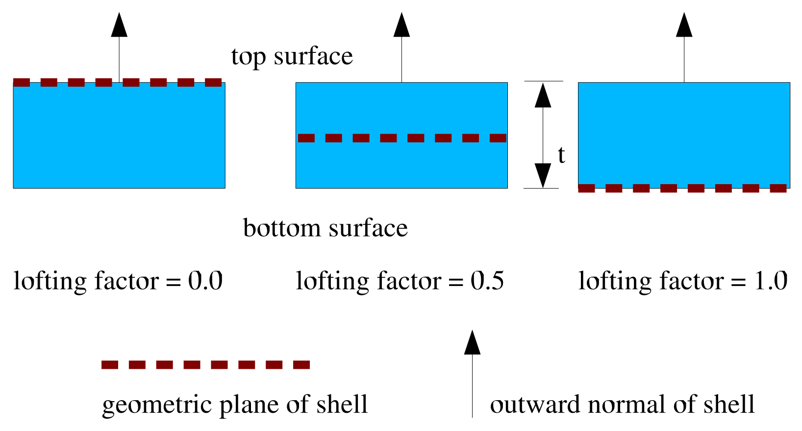
Fig. 6.4 Location of geometric plane of shell for various lofting factors.

Consider the example of a lofting factor set to 1.0 for a shell with thickness of 0.2 inch. In this case, the top surface of the shell will be located at a distance of 0.2 inch from the geometric surface (measuring in the direction of the positive shell normal), and the bottom surface will be located at the geometric surface.

Both the shell mechanics and contact use shell lofting. See Section 8.4 for a discussion of lofting surfaces for shells and contact. It is recommended that shell lofting values other than 0.5 not be used if the shell is thick. If the shell is thicker than its in-plane width, the shell lofting algorithms may become unstable.

Sierra/SM can also initialize the lofting factor using an attribute defined on elements in the mesh file. The lofting factor can be set using any field present on the input mesh. To specify a field other than the single-element attribute, use the following form of the LOFTING FACTOR MESH VARIABLE command line:

LOFTING FACTOR MESH VARIABLE = <string>var_name

Here, the string var_name is the name of the initializing field.

A third, and slightly different way lofting can be implemented is through the command

OFFSET MESH VARIABLE = <string>var_name

which allows an offset value to be read from an attribute (or variable) on the mesh file. This attribute (or variable) must be named but may have any name, and this name is specified in place of var_name in the command. An offset is a dimensional (i.e., not scaled by the shell thickness) value that gives the shell mid-plane shift in the positive shell normal direction. Internal to Sierra/SM the offset value is converted to an equivalent lofting factor by dividing by the initial thickness and adding 0.5. Thus, an offset of zero gives a lofting factor of 0.5, an offset of one half of the thickness gives a lofting factor of one, and an offset of negative one half of the thickness gives a lofting factor of zero. There is no check that given offset values produce lofting values between zero and one, which allows any offset to be specified but requires that care be exercised to avoid unstable lofted shells.

Warning

An offset and a lofting factor may not both be specified in the same shell section. Both determine the shell lofting and may conflict.

The ORIENTATION command line lets the user select a coordinate system for output of in-plane stresses and strains. The ORIENTATION option makes use of an embedded coordinate system \(r,s,t\) associated with each shell element. The \(r,s,t\) coordinate system for a shell element is shown in Fig. 6.5. The \(r\)-axis extends from the center of the shell to the midpoint of the side of the shell defined by nodes 1 and 2. The \(t\)-axis is located at the center of the shell and is normal to the surface of the shell at the center point. The \(s\)-axis is the cross-product of the \(t\)-axis and the \(r\)-axis. The \(r,s,t\)-axes form a local coordinate system at the center of the shell; this local coordinate system moves with the shell element as the element deforms.

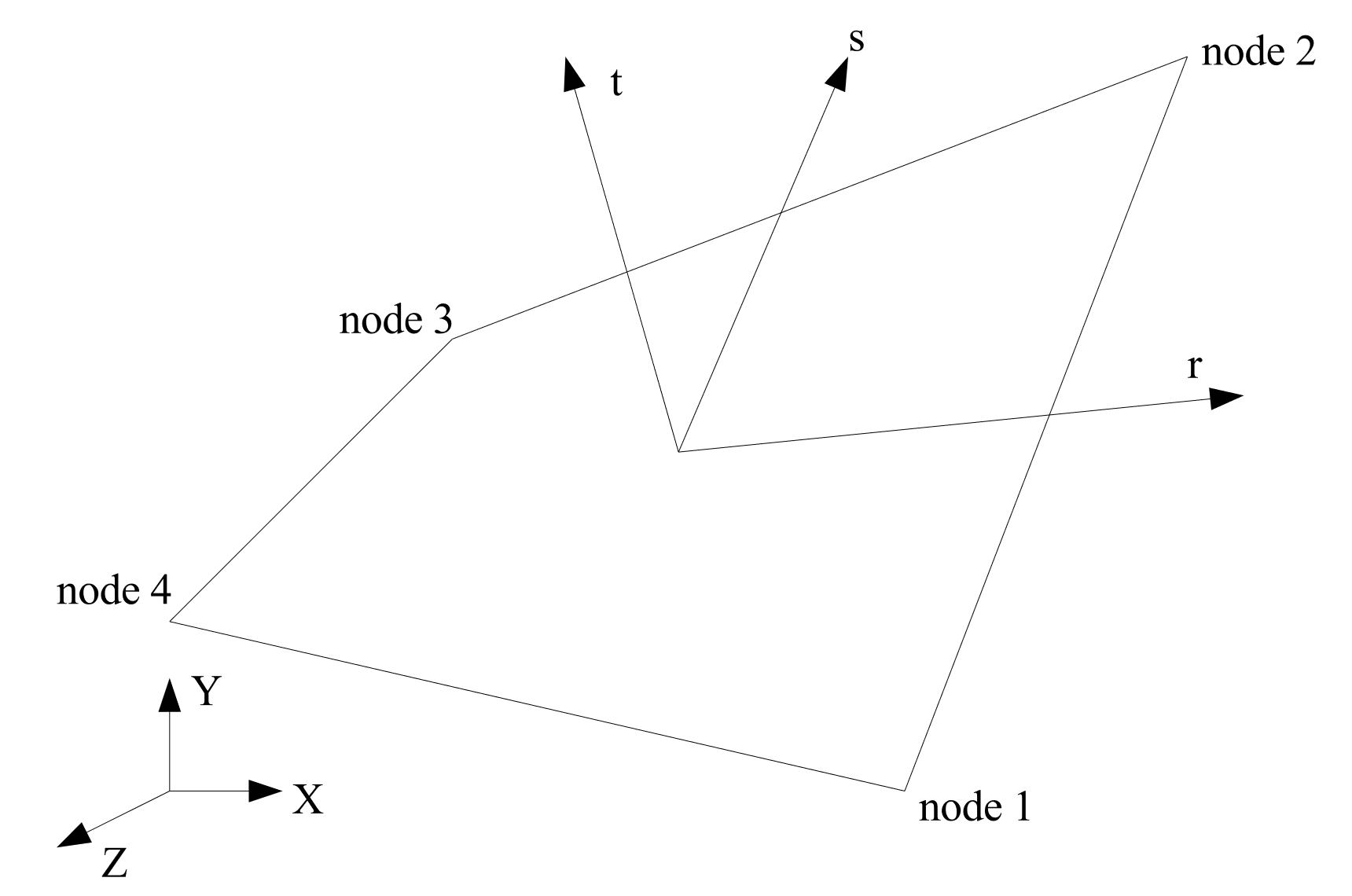
Fig. 6.5 Local \(rst\) coordinate system for a shell element.

The ORIENTATION command line in the SHELL SECTION command block references an ORIENTATION command block that appears in the SIERRA scope. As described in Section 2 of this document, the ORIENTATION command block can be used to define a local co-rotational coordinate system \(X''Y''Z''\) at the center of a shell element. In the original shell configuration (time 0), one of the axes—\(X''\), \(Y''\), or \(Z''\)—is projected onto the plane of the shell element. The angle between this projected axis of the \(X''Y''Z''\) coordinate system and the \(r\)-axis is used to establish the transformation for in-plane stresses and strains. We will illustrate this with an example.

Suppose that in an ORIENTATION command block a rotation of 30 degrees about the 1-axis (\(X'\)-axis) has been specified. The command line for this rotation in the ORIENTATION command block would be

ROTATION ABOUT 1 = 30

For this case, the \(Y''\)-axis is projected onto the plane of the shell (Fig. 6.6). The angle between this projection and the \(r\)-axis establishes a transformation for the in-plane stresses of the shell (the stresses in the center of the shell lying in the plane of the shell). What will be output as the in-plane stress \(\sigma_{xx}^{ip}\) will be in the \(Y''\)-direction; what will be output as the in-plane stress \(\sigma_{yy}^{ip}\) will be in the \(Z''\)-direction. The in-plane stress \(\sigma_{xy}^{ip}\) is a shear stress in the \(Y''Z''\)-plane. The \(X''Y''Z''\) coordinate system maintains the same relative position in regard to the \(rst\) coordinate system. This means that the \(X''Y''Z''\) coordinate system is a local coordinate system that moves with the shell element as the element deforms.

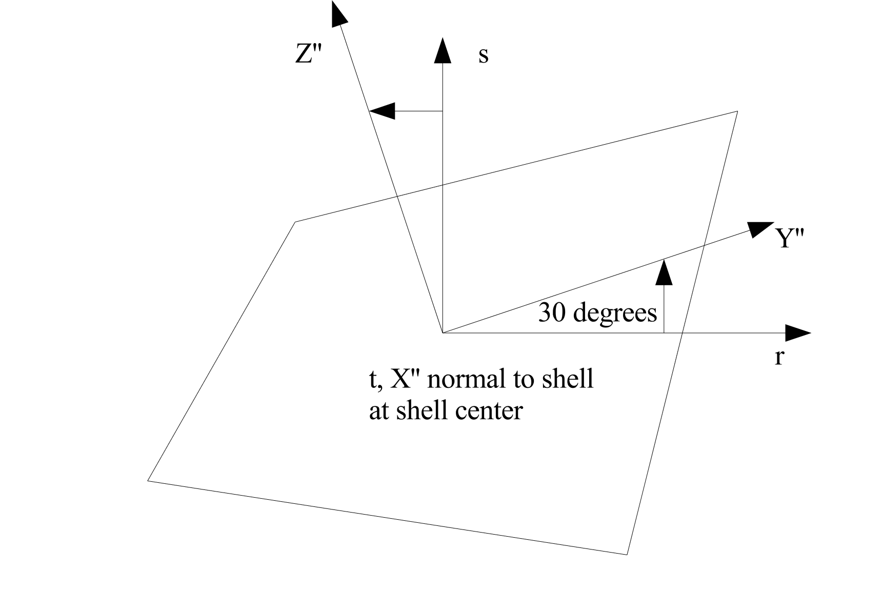
Fig. 6.6 Rotation of 30 degrees about the 1-axis (\(X'\)-axis).

The following permutations for output of the in-plane stresses occur depending on the axis (1, 2, or 3) specified in the ROTATION ABOUT command line:

• Rotation about the 1-axis (\(X'\)-axis): The in-plane stress \(\sigma_{xx}^{ip}\) will be in the \(Y''\)-direction; the in-plane stress \(\sigma_{yy}^{ip}\) will be in the \(Z''\)-direction. The in-plane stress \(\sigma_{xy}^{ip}\) is a shear stress in the \(Y''Z''\)-plane.

• Rotation about the 2-axis (\(Y'\)-axis): The in-plane stress \(\sigma_{xx}^{ip}\) will be in the \(Z''\)-direction; the in-plane stress \(\sigma_{yy}^{ip}\) will be in the \(X''\)-direction. The in-plane stress \(\sigma_{xy}^{ip}\) is a shear stress in the \(Z''X''\)-plane.

• Rotation about the 3-axis (\(Z'\)-axis): The in-plane stress \(\sigma_{xx}^{ip}\) will be in the \(X''\)-direction; the in-plane stress \(\sigma_{yy}^{ip}\) will be in the \(Y''\)-direction. The in-plane stress \(\sigma_{xy}^{ip}\) is a shear stress in the \(X''Y''\)-plane.

If no orientation is specified, the in-plane stresses and strains are output in the consistent axes from a default orientation, which is a rectangular system with the \(X'\) and \(Y'\) axes taken as the global \(X\) and \(Y\) axes, respectively, and ROTATION ABOUT 1 = 0.0.

The command line

DRILLING STIFFNESS FACTOR = <real>stiffness_factor

adds stiffness in the drilling degrees of freedom to quadrilateral shells. Drilling degrees of freedom are rotational degrees of freedom in the direction orthogonal to the plane of the shell at each node. The formulation used for the quadrilateral shells has no rotational stiffness in this direction. This can lead to spurious zero-energy modes of deformation similar in nature to hourglass deformation. This makes obtaining a solution difficult in quasistatic problems and can result in singularities when using the full tangent preconditioner.

The stiffness_factor should be chosen as a quantity small enough to add enough stiffness to allow the solve to be successful without unduly affecting the solution. The default value for stiffness_factor is 1.0e-5, which places drilling stiffness about 10000X lower than the bending stiffness. If singularities are encountered in the solution or hourglass-like deformation is observed in the drilling degrees of freedom, setting a larger value may be appropriate.

Elements in a section can be made rigid by including the RIGID BODY command line. The RIGID BODY command line specifies an indenter that maps to a rigid body command block. See Section 6.3.1 for a full discussion of how to create rigid bodies and Section 6.3.1.1 for information on the use of the RIGID BODIES FROM ATTRIBUTES command.

The command line STABLE TIME STEP ESTIMATE specifies the method used to calculate the size of the critical time step. The default method is GERSCHGORIN circle theorem, which is used to find a bound to the maximum membrane, shear and bending frequencies of the problem. The COURANT method uses the characteristic length of the element and the membrane wave speed to approximate the stable time step. This estimate tends to be less conservative than GERSCHGORIN, but might not be appropriate for problems with dominant shear or bending responses. This command line option is only available for quadrilateral shells. Triangular shells will only use the Courant estimate.

The command lines CONTACT SHELL THICKNESS and CONTACT SHELL LOFTING can be used to set the thickness and lofting factor for use in contact. This can be a different thickness or lofting factor than used for defining the element stiffness.

6.2.5.1. Orthotropic Properties

Orthotropic shell materials define their properties within a characteristic coordinate system. This element-local \(R,S,T\) coordinate system may be defined using the FIBER ORIENTATION, R VECTOR READ VARIABLE, and T VECTOR READ VARIABLE commands. Command lines R VECTOR READ VARIABLE and T VECTOR READ VARIABLE specify the element fields which contain vectors \(R_{\textrm{input}}\) and \(T_{\textrm{input}}\), respectively, used to define this coordinate system, while FIBER ORIENTATION specifies an in-plane rotation of this element-wise coordinate system.

Construction of the local coordinate system, demonstrated graphically in Fig. 6.7, is performed in the undeformed configuration; the coordinate system moves with its associated shell element throughout the analysis. The orientation of \(T_{\textrm{input}}\) determines whether the positive or negative shell normal is selected as the out-of-plane \(T\)-direction. Intermediate direction \(R'\) is computed by projecting \(R_{\textrm{input}}\) into the plane of the shell, such that it is orthogonal to \(T\). The third orthogonal direction is computed as \(S'= T \times R'\). Rotating intermediate directions \(R'\) and \(S'\) about the \(T\)-axis by the specified FIBER ORIENTATION angle \(\Theta\) yields the final local \(R,S,T\) coordinate system. The \(R\), \(S\), and \(T\) directions can be visualized by requesting element fields “r_vector,” “s_vector,” and “t_vector,” respectively, in results output. Additional guidance on the output and visualization of element quantities is available in Section 9.3.

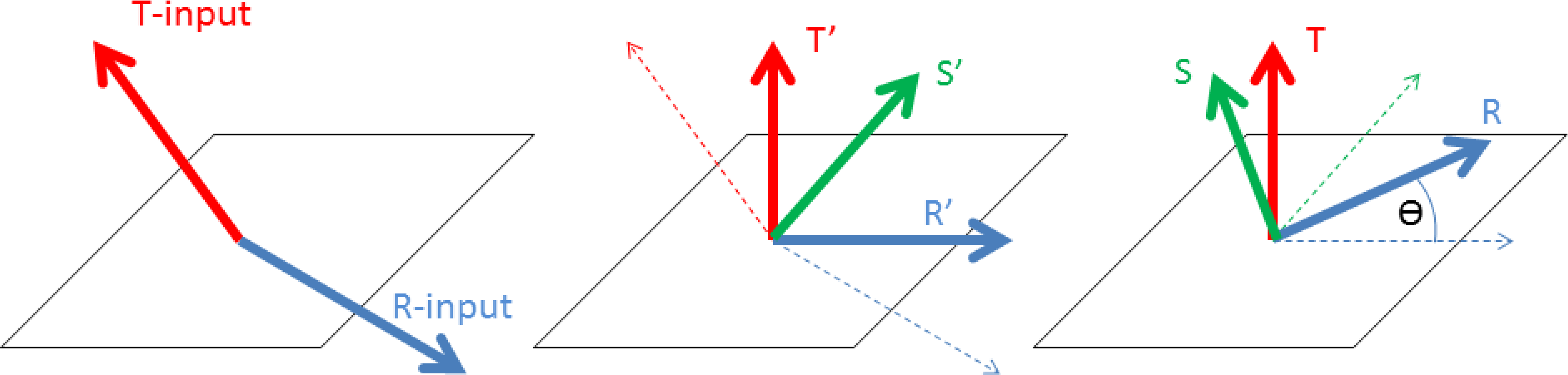
Fig. 6.7 Definition of shell \(R,S,T\) coordinate system.

6.2.6. Layered Shell Section

BEGIN LAYERED SHELL SECTION <string>sect
  LAYER <int>layerId = <string>subSectName
                       <string>material <string>model
  LOFTING FACTOR = <real>loft(0.5)
  CONTACT THICKNESS = <real>contactThickness
  CONTACT LOFTING FACTOR = <real>contactLofting
END

The LAYERED SHELL SECTION command block is used to define a single shell element that is a composite of layers with different properties. The layers of the shell can have different materials and different shell formulations.

Internally to the code a layered shell is represented by several individual elements that share the same nodes and same topology. Layered shells will create new element blocks and new elements in the output file to represent each distinct shell layer. Boundary conditions such as contact or element death can be performed on either the original shell element or on the individual layers specifying the appropriate block name.

The LAYER defines a layer for the current shell. The layers of the shell will be stacked from the bottom to the top based on the order of the LAYER commands on the input deck. A shell may have up to 99 different layers defined. The layerId input is a positive integer provided by the user. This number will be used to label the shell layers to aid in visualization. The new element block sub-layers will be named based on the provided layerId using the convention

<block_name>_SIERRA_CREATED_LAYER<layerID>

The subSectName is the name of the shell section associated with the layer. The shell section will be used to define the thickness of the layer and any shell formulation options to use in the layer. The material and model names define the material and material model that the layer is composed of. Any material that is valid for shell elements can be used as a shell layer material. A default material and model may be provided in the parameters for block command block. Any layer in the section that does not define a material and model will use this default material and model.

Note that the first order approximations used in the shell element formulation does not accurately compute transverse shear strains for layered shells. This is handled and corrected internally by applying a shear correction factor [[10]].

The lofting factor for the entire shell stack can be specified with the LOFTING FACTOR option. Similar to standard shells this lofting factor can vary from 0.0 to 1.0 and has a default value of 0.5 (shell element passes through mid-plane of the layered shell stack.) The lofting of the individual layers will be computed automatically based on the layer thicknesses and layered shell lofting factor.

The command lines CONTACT SHELL THICKNESS and CONTACT SHELL LOFTING can be used to set the thickness and lofting factor for use in contact. These commands define the contact behavior of the layered shell stack as a whole.

Example of layered shell syntax:

begin shell section SHELL_1
  thickness = 0.1
end shell section SHELL_1

begin shell section SHELL_2
  thickness = 0.2
end shell section SHELL_2

begin shell section SHELL_3
  thickness = 0.1
end shell section SHELL_3

begin layered shell section LAYERED_SHELL
  layer 1 = SHELL_1 steel  elastic
  layer 2 = SHELL_2 copper elastic_plastic
  lofting factor = 1.0
end

begin parameters for block block_1
  section = LAYERED_SHELL
end

In the above example a two layer shell is defined. The composite shell has thickness of 0.3. The bottom layer of the shell is made of elastic steel with a thickness of 0.1. On top of the steel is a 0.2 thick layer of elastic plastic copper. The entire layer stack-up has a lofting factor of 1.0 with respect to the shell element. The configuration is shown in Fig. 6.8. The layer specific resultants on the different shell layers can be seen by looking in the results output file element blocks named block_1_SIERRA_CREATED_LAYER_1 and block_1_SIERRA_CREATED_LAYER_2.

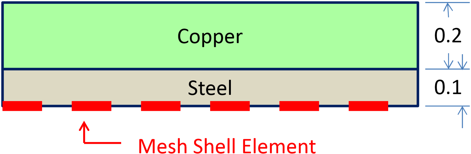
Fig. 6.8 Layered shell example.

6.2.7. Membrane Section

BEGIN MEMBRANE SECTION <string>membrane_section_name
  THICKNESS = <real>mem_thickness
  THICKNESS MESH VARIABLE =
    <string>THICKNESS|<string>var_name
  THICKNESS TIME STEP = <real>time_value
  THICKNESS SCALE FACTOR = <real>thick_scale_factor(1.0)
  CONTACT THICKNESS SCALE FACTOR = <real>thick_scale_factor(thick_scale_factor)
  FORMULATION = <string>MEAN_QUADRATURE|
    SELECTIVE_DEVIATORIC(MEAN_QUADRATURE)
  DEVIATORIC PARAMETER = <real>deviatoric_param
  LOFTING FACTOR = <real>lofting_factor(0.5)
  LOFTING FACTOR MESH VARIABLE = <string>var_name
  RIGID BODY = <string>rigid_body_name
  RIGID BODIES FROM ATTRIBUTES = <integer>first_id
    TO <integer>last_id
  CONTACT THICKNESS = <real>contactThickness
  CONTACT LOFTING FACTOR = <real>contactLofting
END [MEMBRANE SECTION <string>membrane_section_name]

The MEMBRANE SECTION command block specifies the properties for a membrane element. If a section defined by this command block is referenced in the parameters for a block of four-noded elements, the elements in that block will be treated as membranes. The parameter membrane_section_name is user-defined and is referenced by a SECTION command line in a PARAMETERS FOR BLOCK command block.

Either a THICKNESS command line or a THICKNESS MESH VARIABLE command line must appear in the MEMBRANE SECTION command block.

If a membrane element block references a MEMBRANE SECTION command block with the command line

THICKNESS = <real>mem_thickness

then all the membrane elements in the block will have their thickness initialized to the value mem_thickness.

Sierra/SM can also initialize the thickness using an attribute defined on elements in the mesh file. Meshing programs such as PATRAN and CUBIT typically set the element thickness as an attribute on the elements. If the elements have one and only one attribute defined on the mesh, the THICKNESS MESH VARIABLE command line should be specified as

THICKNESS MESH VARIABLE = THICKNESS

which causes the thickness of the element to be initialized to the value of the attribute for that element. If there are zero attributes or more than one attribute, the thickness variable will not be automatically defined, and the command will fail.

The thickness may also be initialized by any other field present on the input mesh. To specify a field other than the single-element attribute, use this form of the THICKNESS MESH VARIABLE command line:

THICKNESS MESH VARIABLE = <string>var_name

where the string var_name is the name of the initializing field.

The input mesh may have values defined at more than one point in time. To choose the point in time in the mesh file that the variable should be read, use the command line:

THICKNESS TIME STEP = <real>time_value

The default time point in the mesh file at which the variable is read is 0.0.

Once the thickness of a membrane element is initialized by using either the THICKNESS command line or the THICKNESS MESH VARIABLE command line, this initial thickness value can then be scaled by using the scale factor command line:

THICKNESS SCALE FACTOR = <real>thick_scale_factor

If the initial thickness of the membrane is 0.15 units, and the value for thick_scale_factor is 0.5, then the scaled thickness of the membrane will be 0.075 units.

CONTACT THICKNESS SCALE FACTOR = <real>contact_thick_scale_factor

The CONTACT THICKNESS SCALE FACTOR command is used for overwriting the value of THICKNESS SCALE FACTOR for contact purposes.

If the initial thickness of the membrane is 0.15 inch, the value of thick_scale_factor is 0.5, and the value of contact_thick_scale_factor is 1.0, then the membrane contact thickness will be equal to the original thickness (0.15) inches.

The FORMULATION command line specifies whether the element will use a single-point integration rule (mean quadrature) or a selective-deviatoric integration rule:

FORMULATION = <string>MEAN_QUADRATURE|SELECTIVE_DEVIATORIC
  (MEAN_QUADRATURE)

If the user wishes to use the selective-deviatoric rule, the DEVIATORIC PARAMETER command line must also appear in the MEMBRANE SECTION command block:

DEVIATORIC PARAMETER = <real>deviatoric_param

The selective-deviatoric elements, when used with a parameter greater than 0.0, provide hourglass control without artificial hourglass parameters. The selective-deviatoric parameter, deviatoric_param, which is valid from 0.0 to 1.0, indicates how much of the deviatoric response should be taken from a uniform-gradient integration and how much should be taken from a full integration of the element. A value of 0.0 will give a pure uniform-gradient response with no hourglass control. Thus, this value is of little practical use. A value of 1.0 will give a fully integrated deviatoric response. Although any value between 0.0 and 1.0 is perfectly valid, lower values are generally preferred.

The command line

LOFTING FACTOR = <real>lofting_factor(0.5)

allows the user to shift the location of the mid-surface of a membrane element relative to the geometric location of the membrane element. By default, the geometric location of a membrane element in a mesh represents the mid-surface of the membrane. If a membrane has a thickness of 0.2 inch, the top surface of the membrane is 0.1 inch above the geometric surface defined by the membrane element, and the bottom surface of the membrane is 0.1 inch below the geometric surface defined by the membrane element. (The top surface of the membrane is the surface with a positive element normal; the bottom surface of the membrane is the surface with a negative element normal.)

Fig. 6.4 illustrates shell lofting, which is also applicable to membranes. For membranes, Fig. 6.4 represents an edge-on view of membrane elements with a thickness of \(t\) and the location of the geometric plane in relation to the membrane surfaces for three different values of the lofting factor—0.0, 0.5, and 1.0. For a lofting factor of 0.0, the geometric surface defined by the membrane corresponds to the top surface of the membrane element. A lofting factor of 1.0 puts the geometric surface at the bottom surface of the membrane element. The geometric surface is midway between the top and bottom surfaces for a lofting factor of 0.5, which is the default.

Consider the example of a lofting factor set to 1.0 for a membrane with thickness of 0.2 inch. In this case, the top surface of the membrane will be located at a distance of 0.2 inch from the geometric surface (measuring in the direction of the positive shell normal), and the bottom surface will be located at the geometric surface.

Both the membrane mechanics and contact use membrane lofting. See Section 8.4 for a discussion of lofting surfaces for membranes and contact.

Sierra/SM can also initialize the lofting factor using an attribute defined on elements in the mesh file. The lofting factor can be set using any field present on the input mesh. To specify a field other than the single-element attribute, use the following form of the LOFTING FACTOR MESH VARIABLE command line:

LOFTING FACTOR MESH VARIABLE = <string>var_name

Here, the string var_name is the name of the initializing field.

Elements in a section can be made rigid by including the RIGID BODY command line. The RIGID BODY command line specifies an indenter that maps to a rigid body command block. Consult Section 6.3.1 for a full description of how to create rigid bodies and Section 6.3.1.1 for information on the use of the RIGID BODIES FROM ATTRIBUTES command.

The command lines CONTACT SHELL THICKNESS and CONTACT SHELL LOFTING can be used to set the thickness and lofting factor for use in contact. The thickness used for contact can be different that the thickness used for the element stiffness calculations.

6.2.8. Beam Section

BEGIN BEAM SECTION <string>beam_section_name
  SECTION = ROD|TUBE|BAR|BOX|I|L|T|T1|C1|C2|Z|HAT|I2
  #
  #  Section dimensions, definition depends on particular section type.
  #
  D1 = <real>d1
  D1 VARIABLE = <STRING>d1_var
  D2 = <real>d2
  D2 VARIABLE = <STRING>d2_var
  D3 = <real>d3
  D3 VARIABLE = <STRING>d3_var
  D4 = <real>d4
  D4 VARIABLE = <STRING>d4_var
  D5 = <real>d5
  D5 VARIABLE = <STRING>d5_var
  D6 = <real>d6
  D6 VARIABLE = <STRING>d6_var

  T AXIS = <real>tx <real>ty <real>tz
  T AXIS VARIABLE = <string>t_axis_var
  REFERENCE AXIS = <string>CENTER|RIGHT|
    TOP|LEFT|BOTTOM(CENTER)
  AXIS OFFSET = <real>s_offset <real>t_offset
  AXIS OFFSET GLOBAL = <real>x_offset <real>y_offset <real>z_offset
  AXIS OFFSET VARIABLE = <string>axis_offset_var
  RIGID BODY = <string>rigid_body_name
  RIGID BODIES FROM ATTRIBUTES = <integer>first_id
    TO <integer>last_id
  VISUALIZE INTEGRATION POINTS = OFF|ON(OFF)
  ROTATIONAL MASS SCALING = OFF|ON(ON)    
END [BEAM SECTION <string>beam_section_name]

The BEAM SECTION command block specifies the properties for a beam element. If this command block is referenced in an element block of three-dimensional, two-node elements, the elements in the block will be treated as beam elements. The name, beam_section_name, can be used by the SECTION command line in a PARAMETERS FOR BLOCK command block.

One of several different types of beam cross section shapes may be specified with the SECTION command. The geometry of each section is defined by up to six geometric parameters, d1 through d6. Some sections require all six parameters some as few as two. If a command of the form D1 = <real>d1 is used the d1 dimension will be constant for all elements in an element block. If a command of the form D1 VARIABLE = <STRING>d1_var the d1 dimension will be read from the mesh file from the element variable named d1_var. When using the DN VARIABLE commands the dimension can be different on every element allowing modeling of tapered beams or other similar structures.

All dimensions used by the beam cross section must be defined in the input deck. If a given beam section geometry requires \(d\) dimensions then that dimension must be specified with exactly one DN = command or DN VARIABLE = command.

The following beam cross sectional geometries are supported:

• ROD: Solid circular or elliptical section. See Fig. 6.9.

• TUBE: Thin walled circular or elliptical tube section. See Fig. 6.10.

• BAR: Sold rectangular section. See Fig. 6.11.

• BOX: Thin walled rectangular section. See Fig. 6.12. D3 is constant for all four walls.

• I: Standard symmetric I beam section. See Fig. 6.13. Width of both flanges given by D4 width of the web given by {D3}.

• L: Thin walled L section. See Fig. 6.14.

• C1: Thin walled C section with open side oriented towards the \(s\) axis. See Fig. 6.15.

• C2: Thin walled C section with open side oriented towards the \(t\) axis. See Fig. 6.16.

• T: Thin walled T section with web oriented along the \(t\) axis. See Fig. 6.17.

• T1: Thin walled T section with web oriented along the \(s\) axis. See Fig. 6.18.

• Z: Thin walled Z section. See Fig. 6.19.

• HAT: Thin walled hat section. See Fig. 6.20. All plates of the same thickness D4.

• I2: Asymmetric I beam section. See Fig. 6.21. The widths and thickness of the two flanges may be specified independently for this section.

Many sections (all but the ROD and BAR) have numerical integration schemes that assume thin walls. This means there is only a single integration point through the thickness of the beam flanges, plates, webs, walls, etc. If a thin walled beam section is defined with plate thickness that are relatively thick compared to the overall beam width and height the numerical properties of the beam may be inaccurate. Specifically the thin walled formulation will tend to underestimate the bending torsional stiffness and strength of thick walled beams.

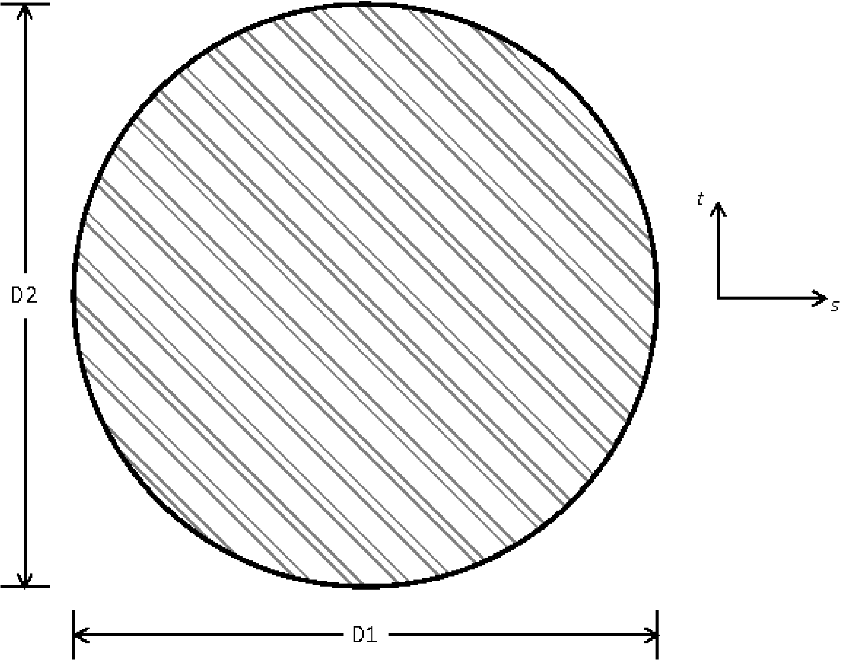
Fig. 6.9 Beam ROD cross section.

Fig. 6.10 Beam TUBE cross section.

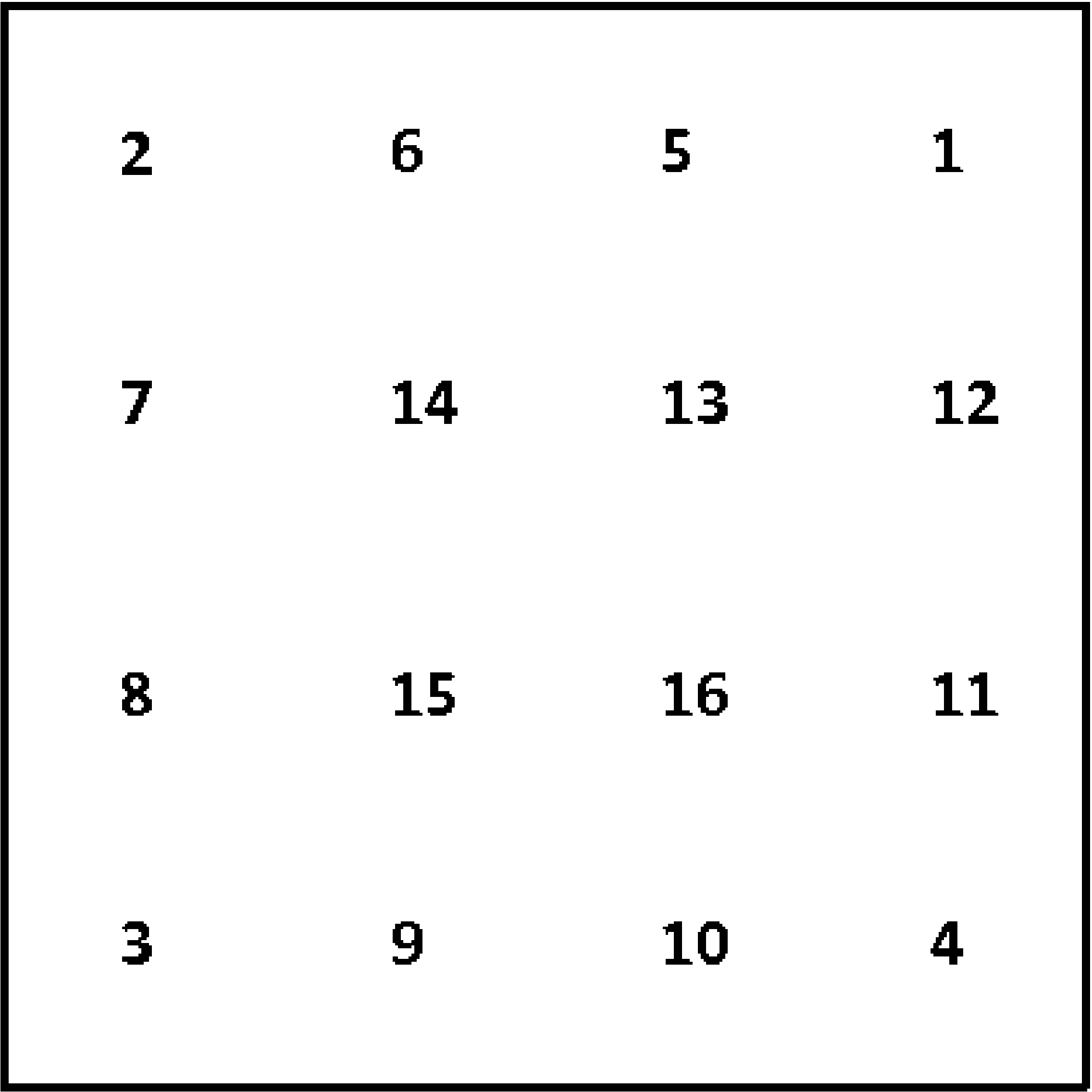
Fig. 6.11 Beam BAR cross section.

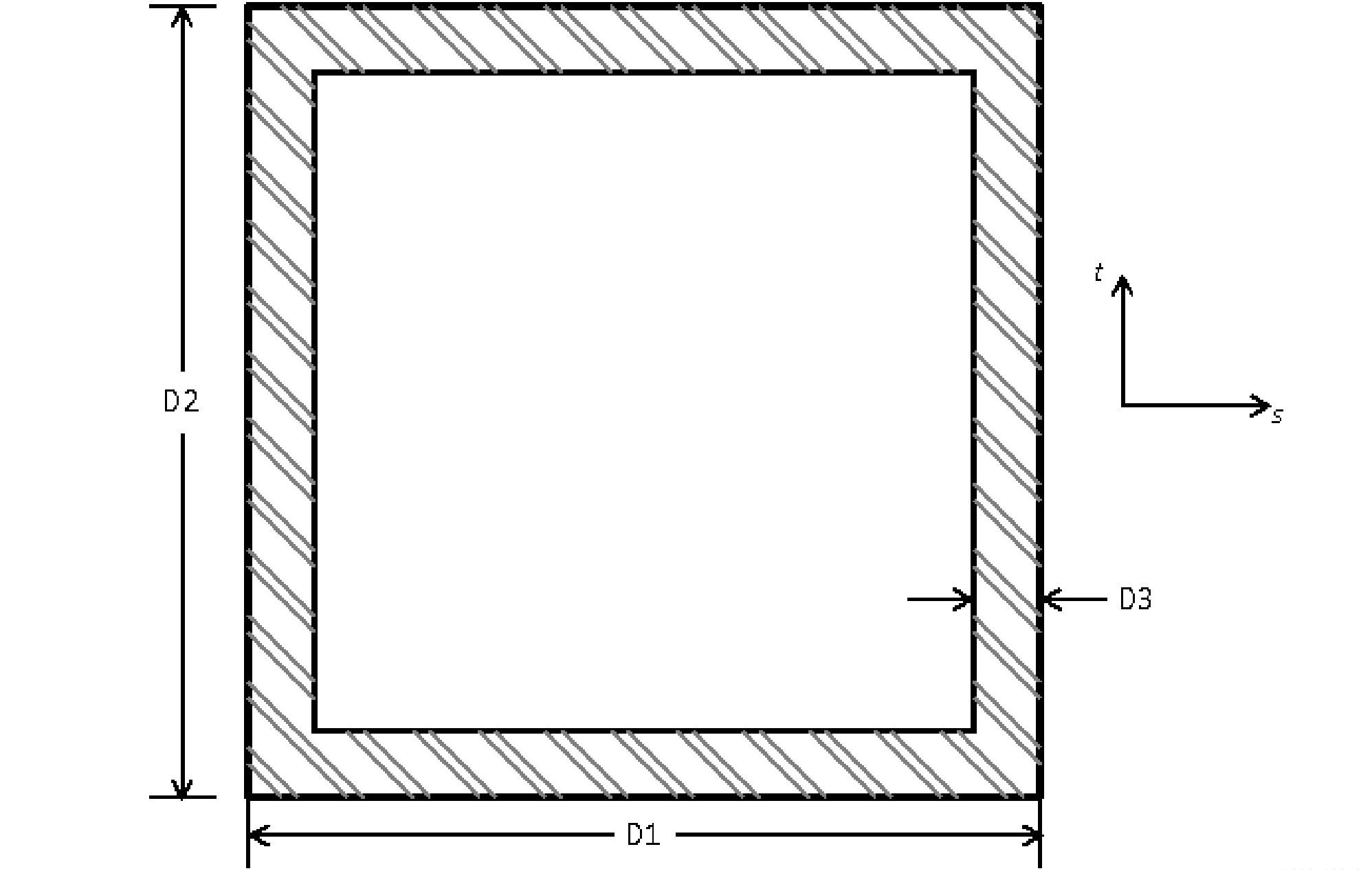
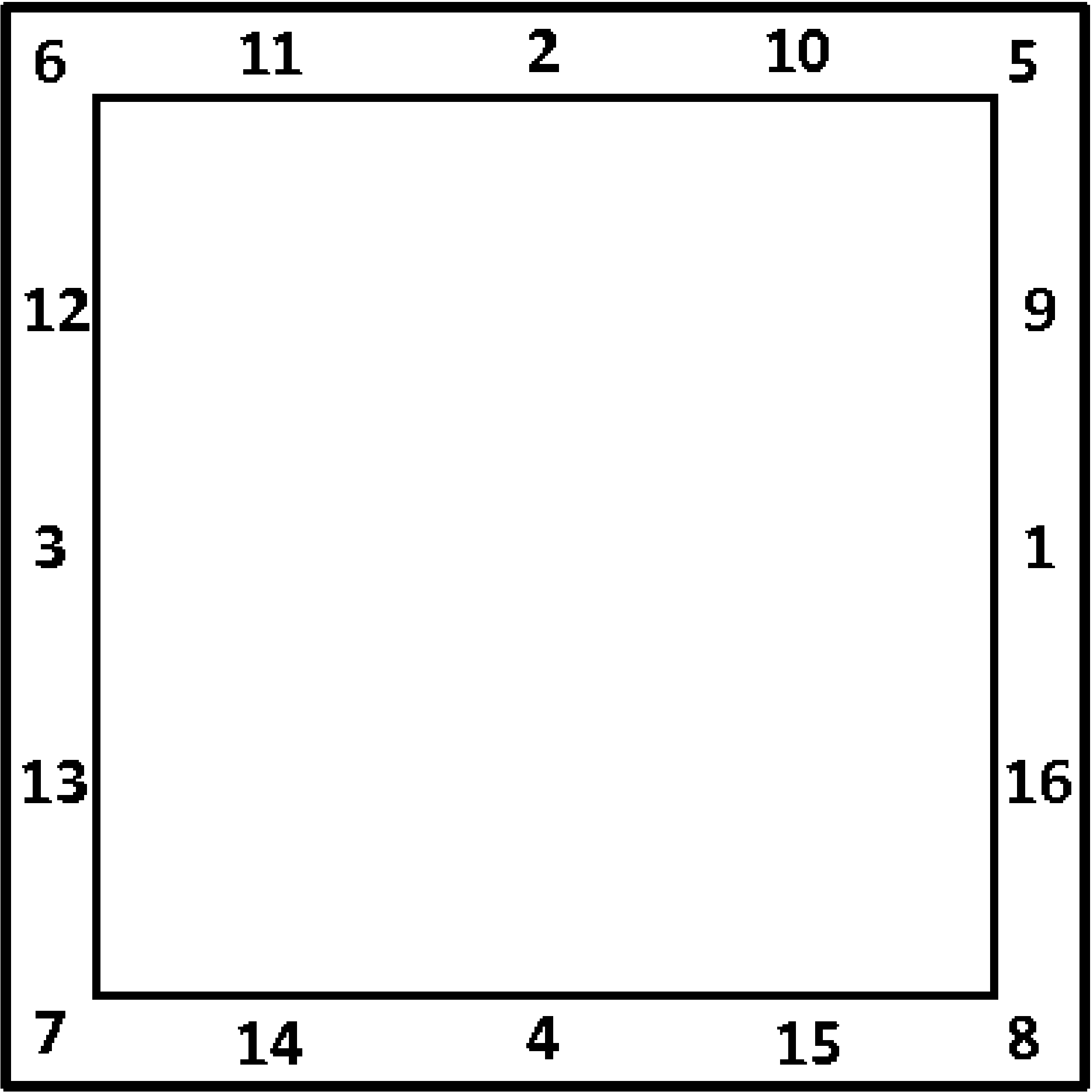
Fig. 6.12 Beam BOX cross section.

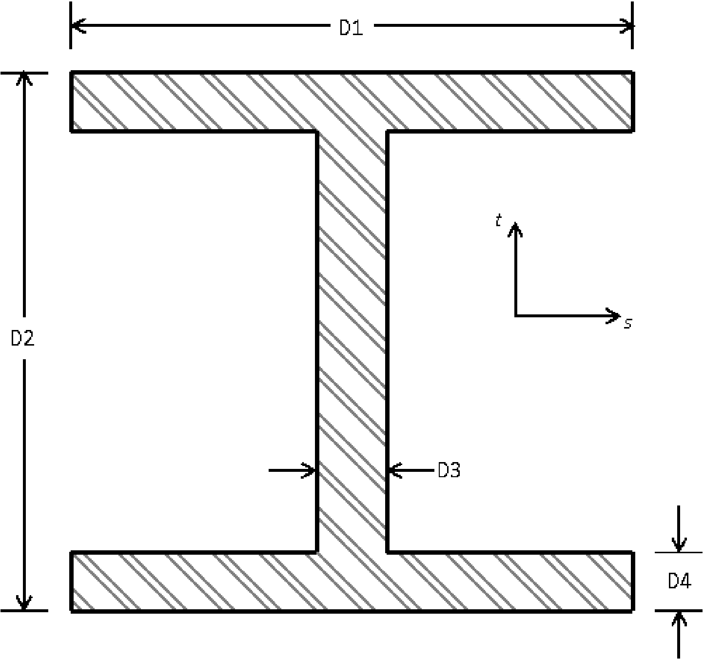
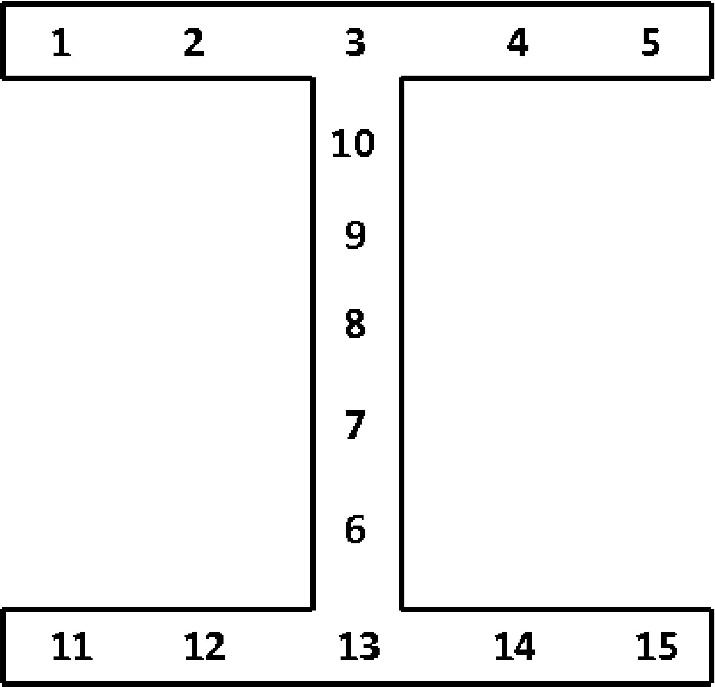
Fig. 6.13 Beam I cross section.

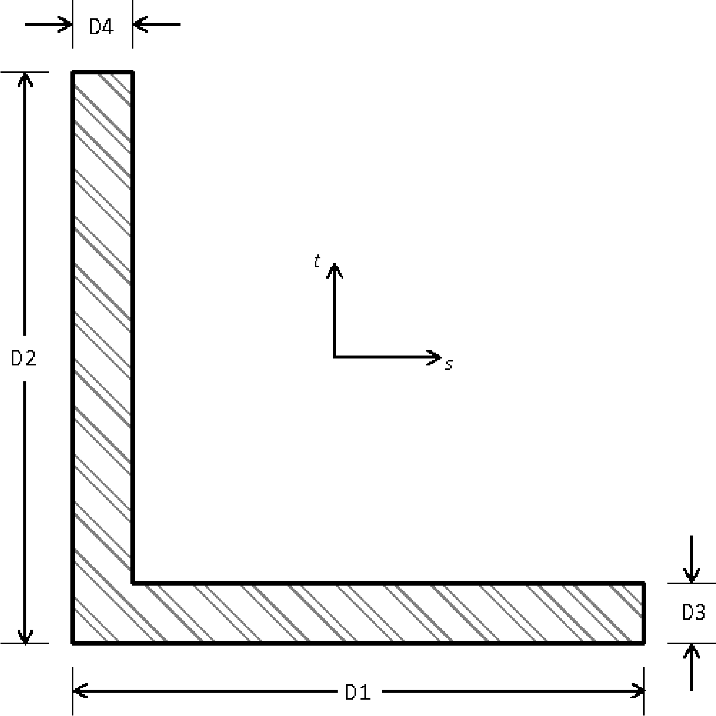
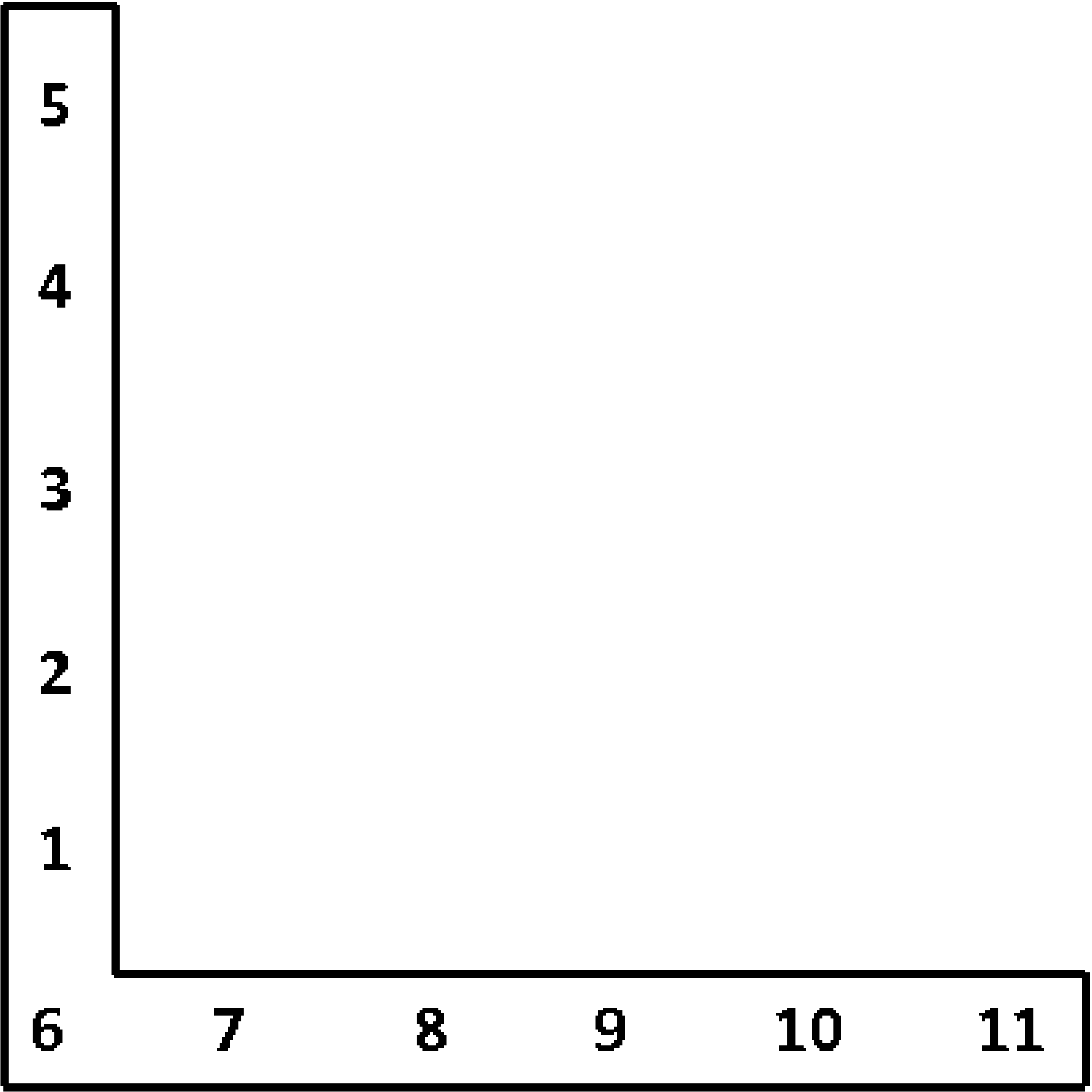
Fig. 6.14 Beam L cross section.

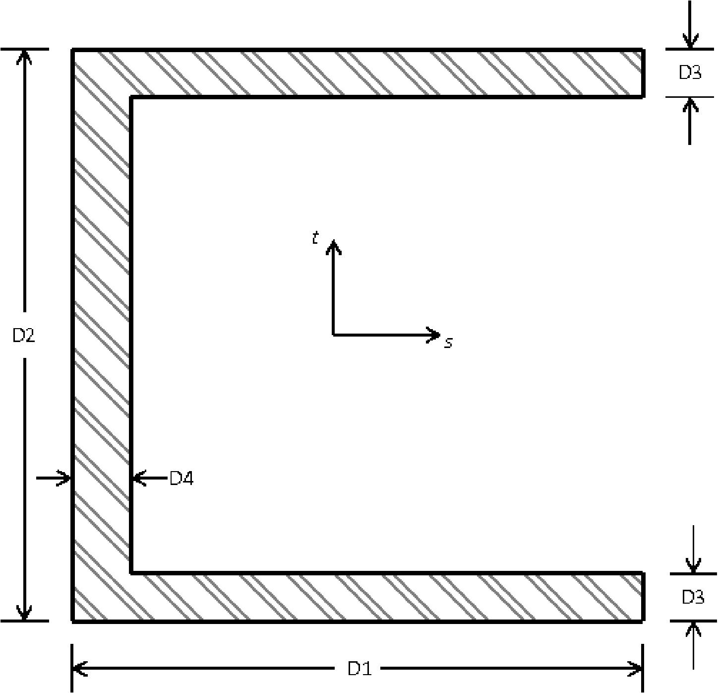
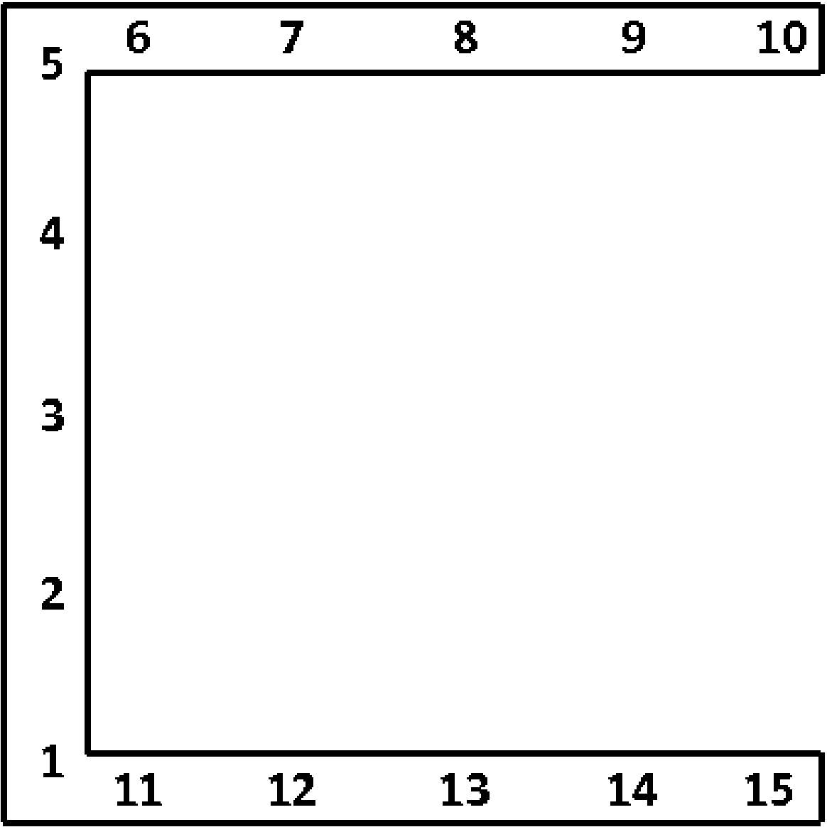
Fig. 6.15 Beam C1 cross section.

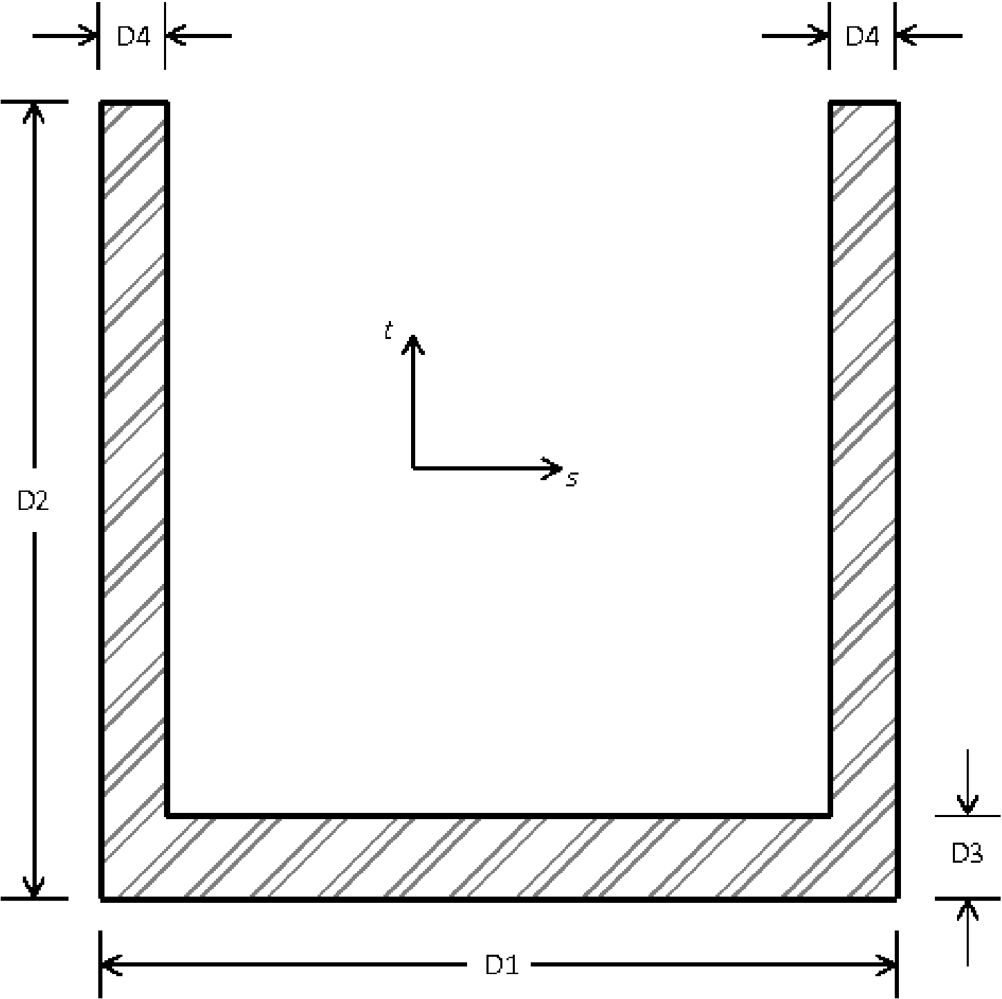
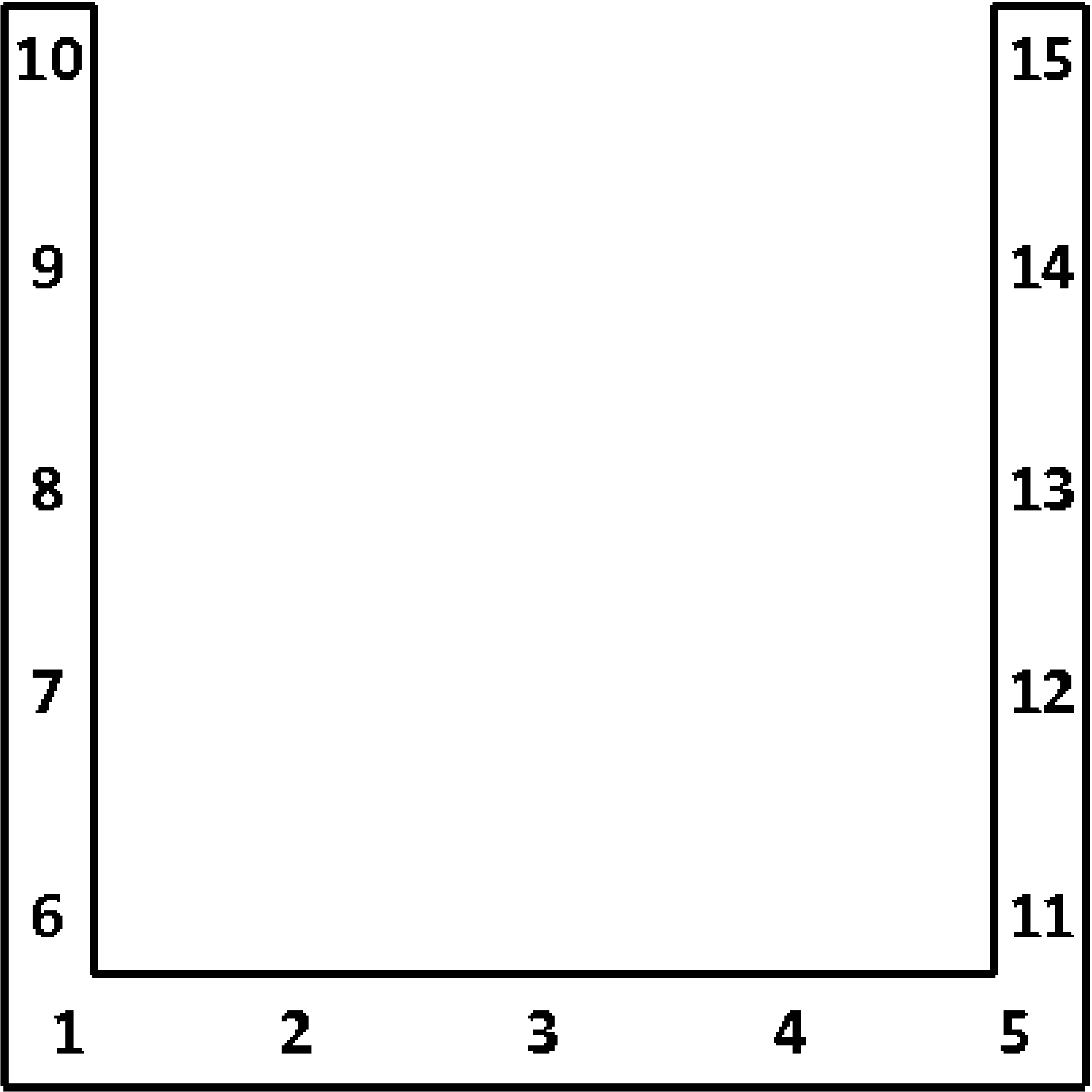
Fig. 6.16 Beam C2 cross section.

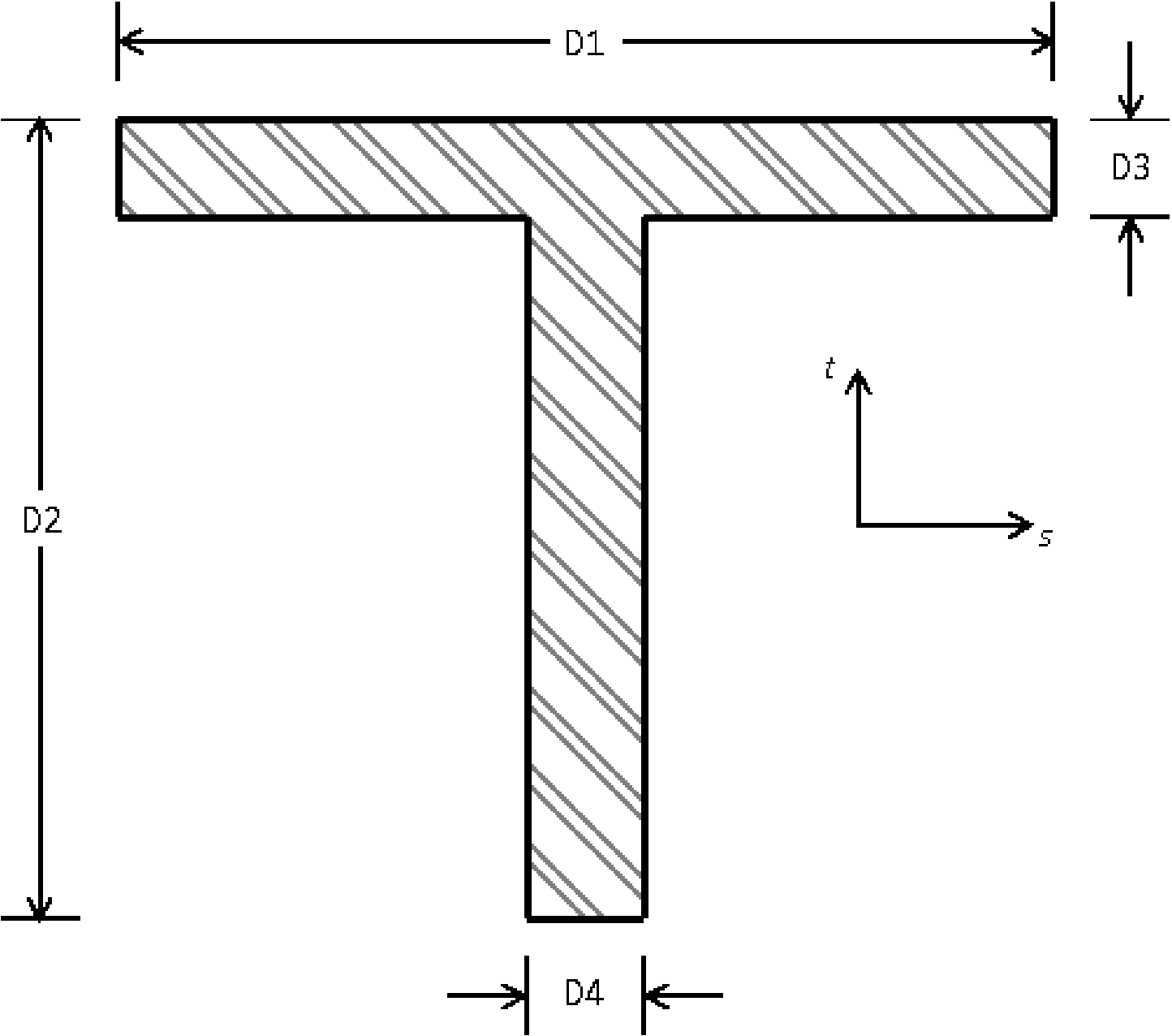
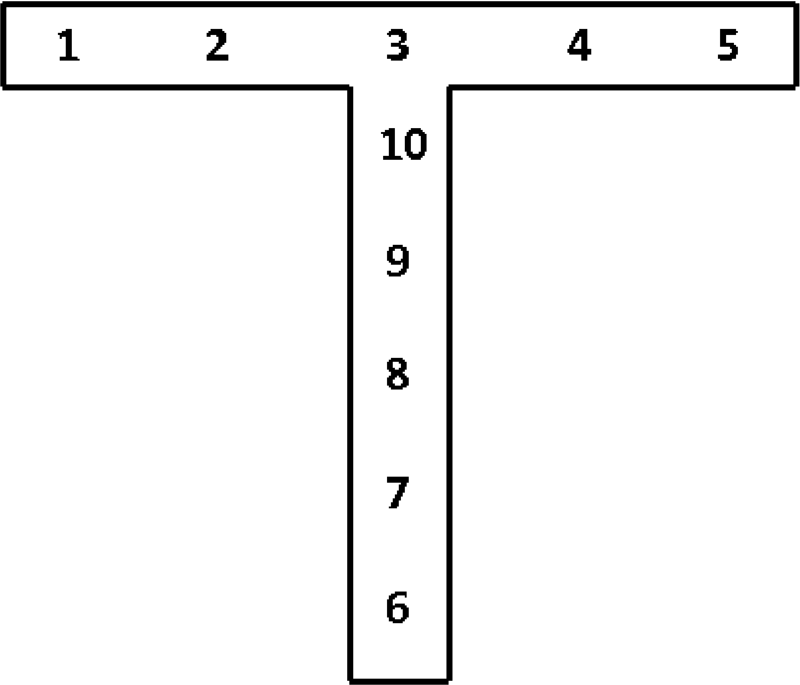
Fig. 6.17 Beam T cross section.

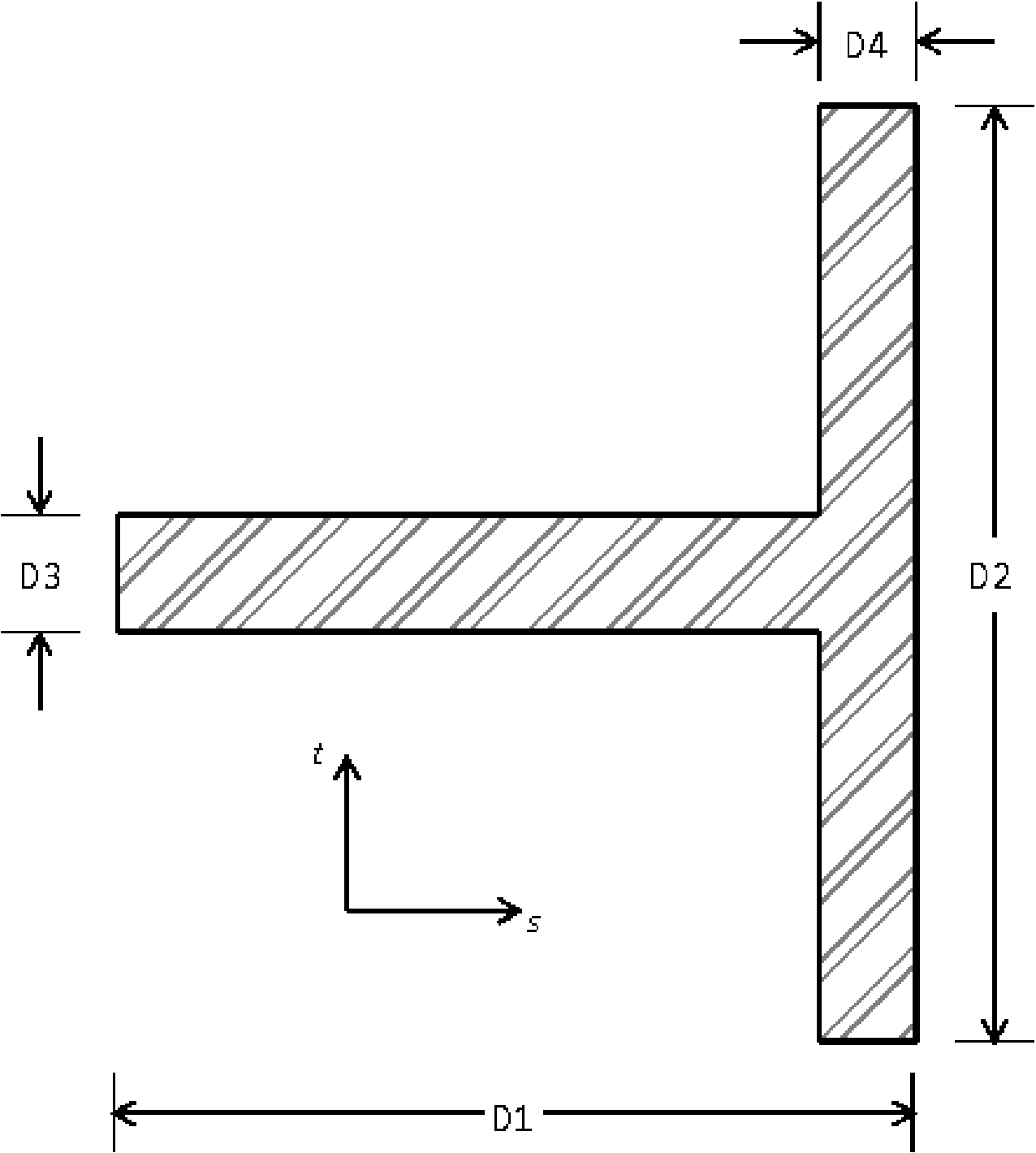
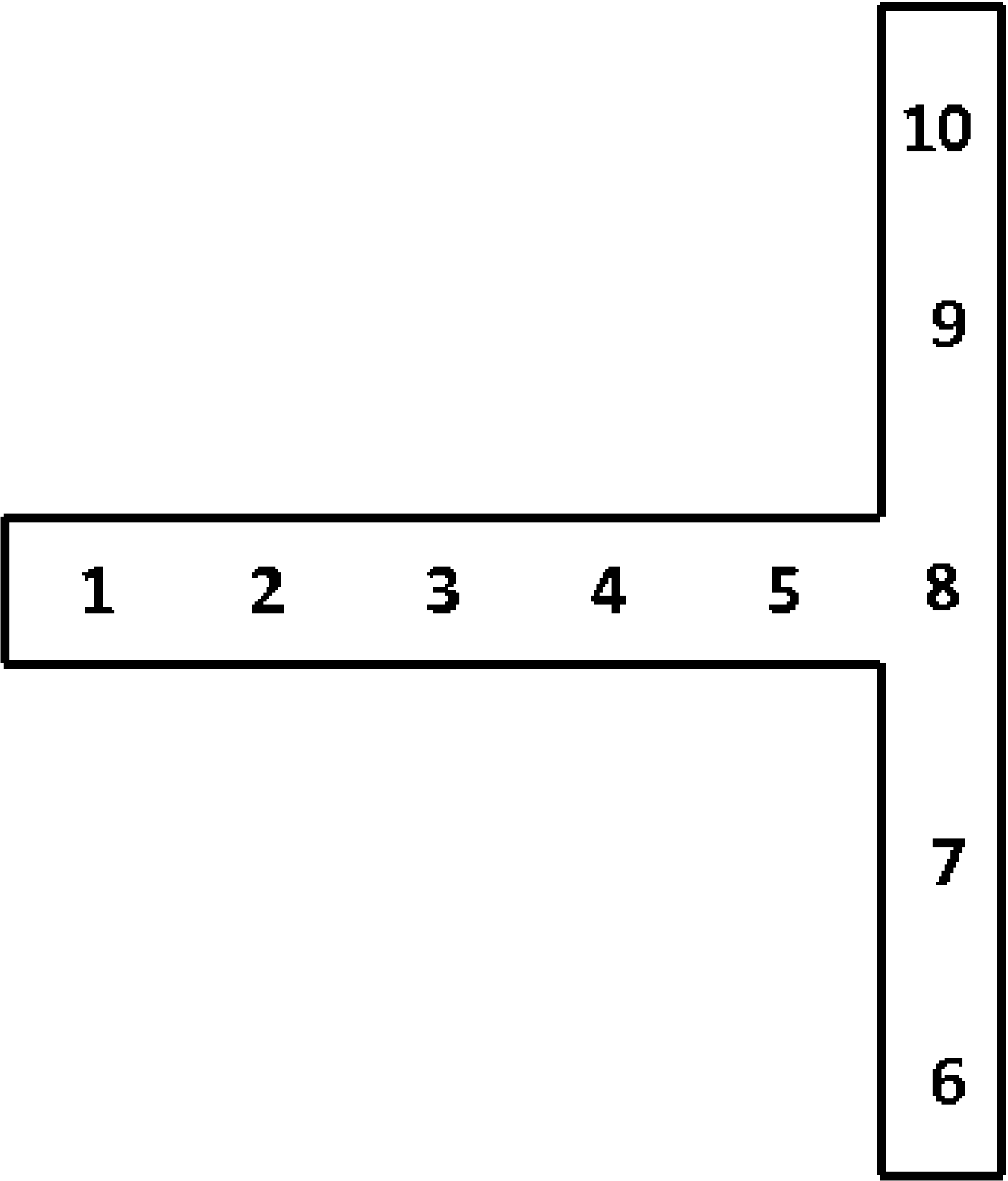
Fig. 6.18 Beam T1 cross section.

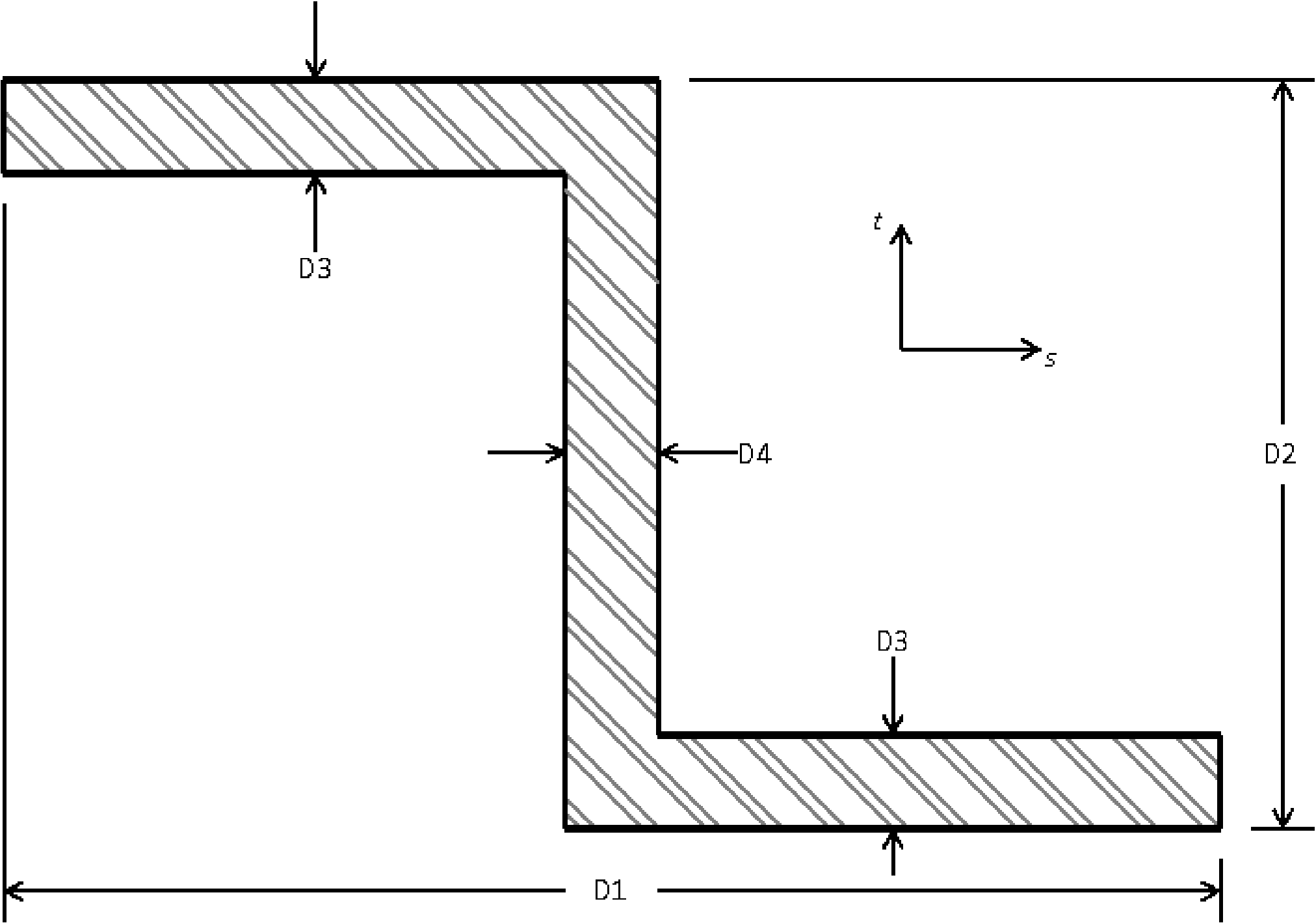
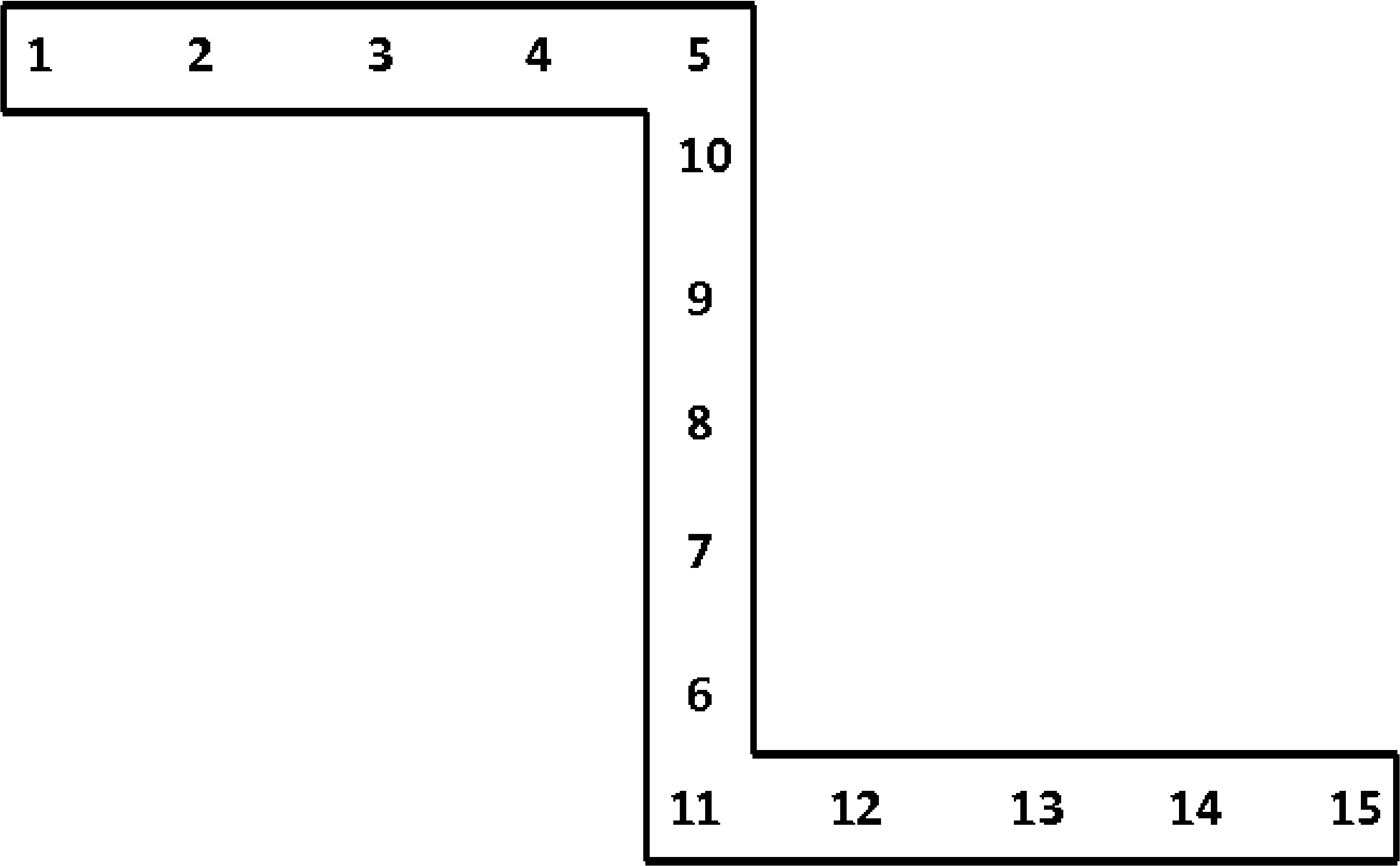
Fig. 6.19 Beam Z cross section.

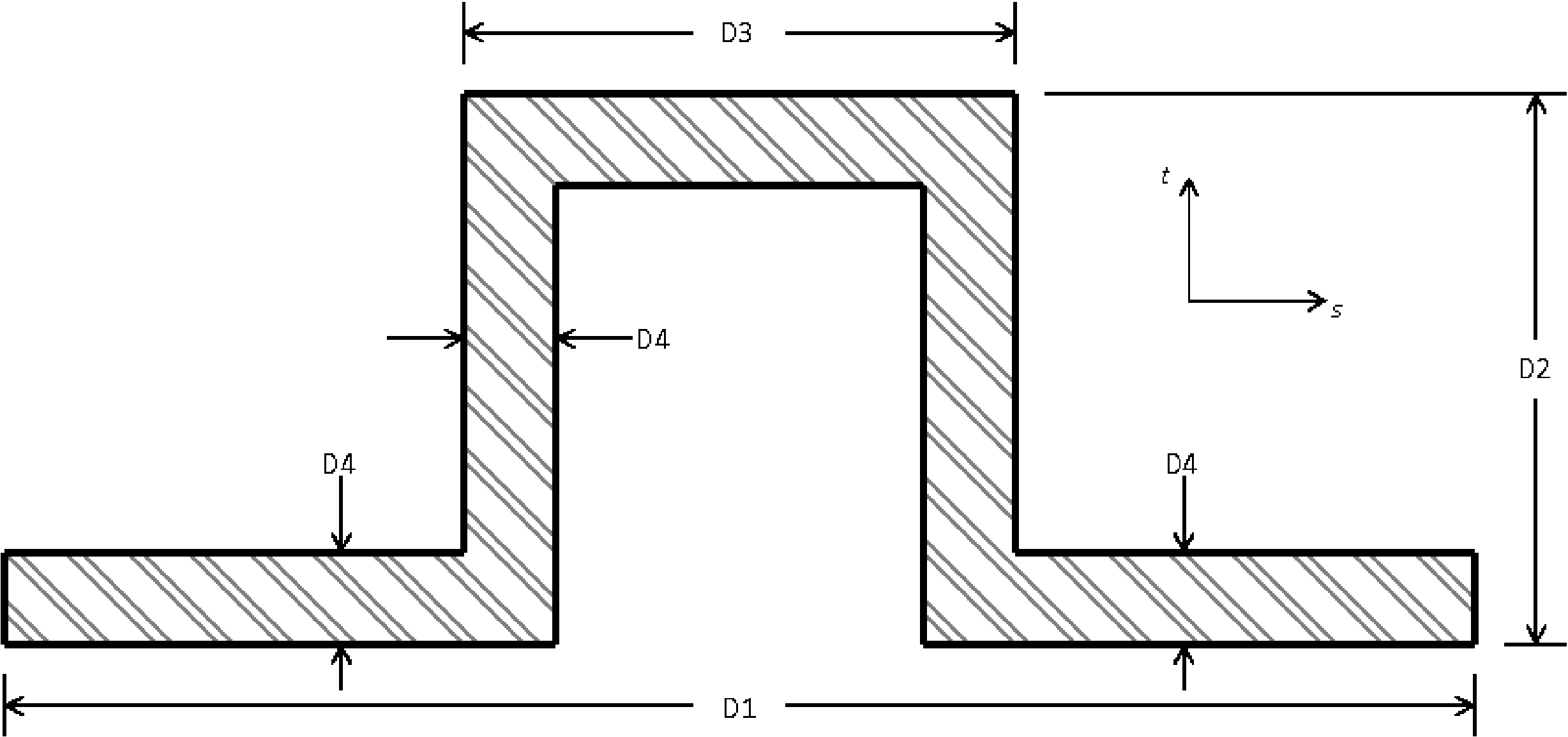
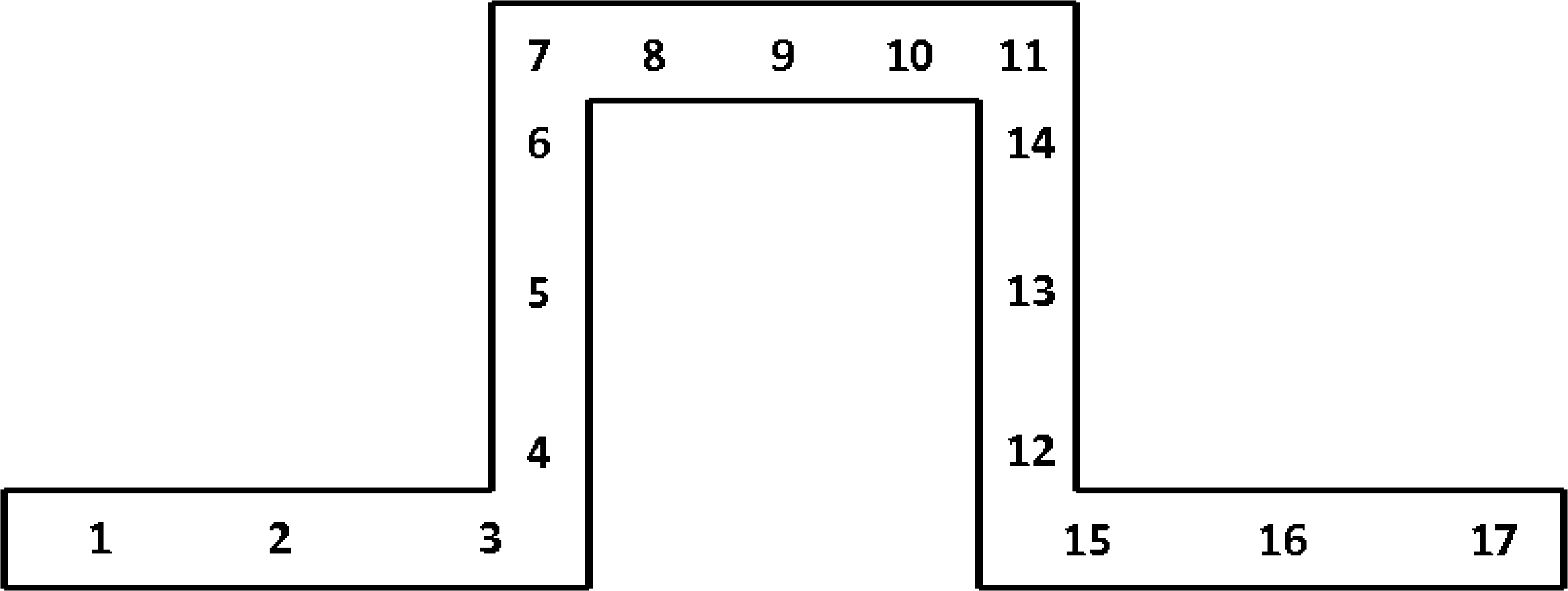
Fig. 6.20 Beam HAT cross section.

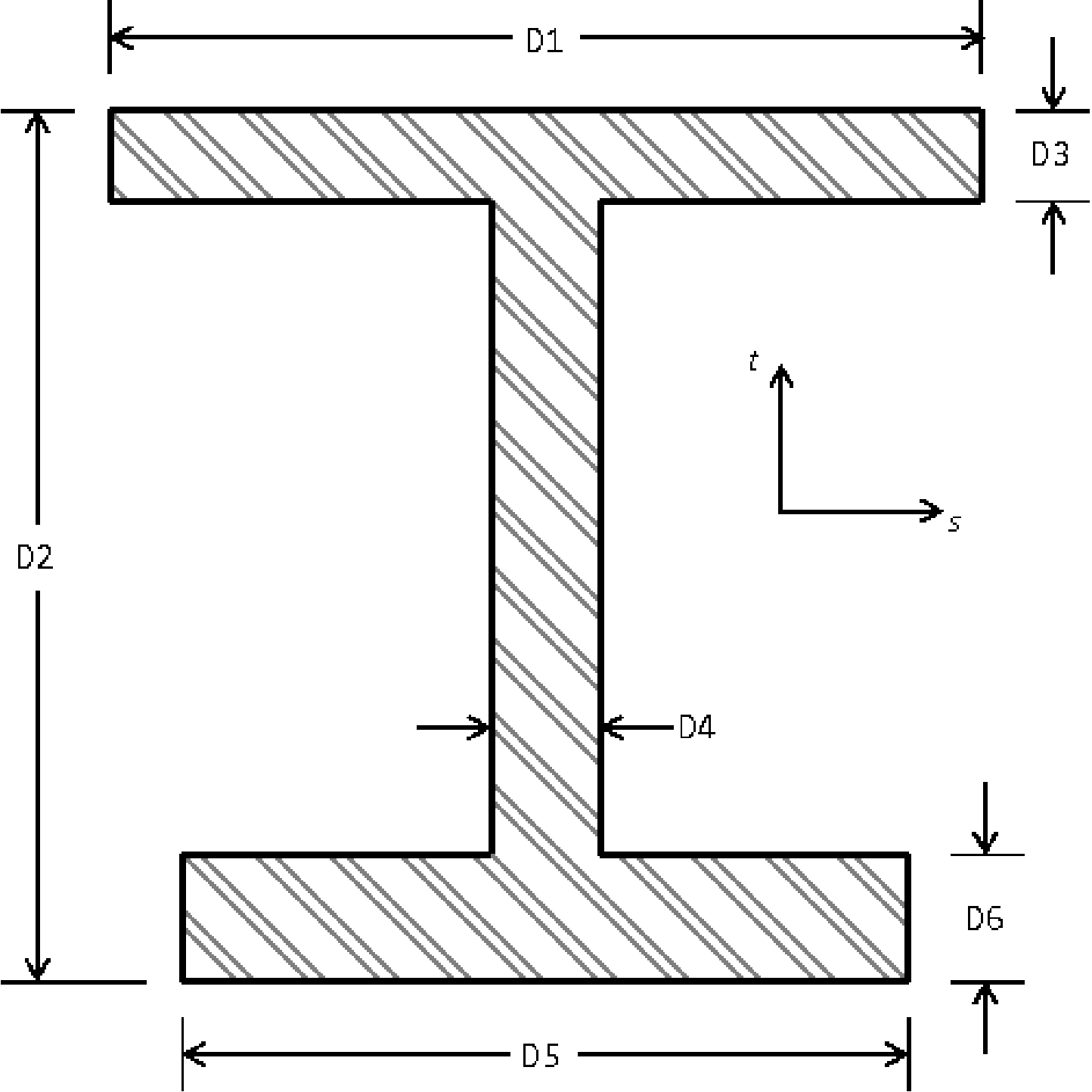
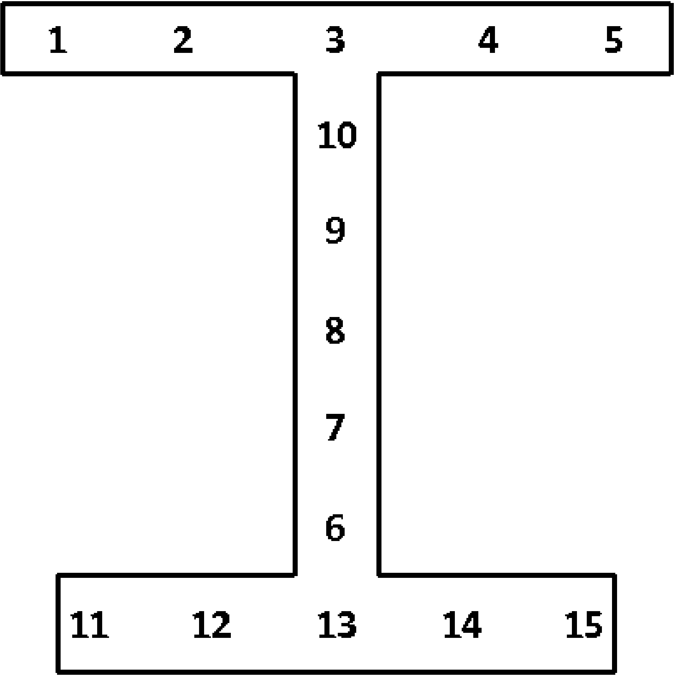
Fig. 6.21 Beam I2 cross section.

Most of the sections require the T AXIS or T AXIS VARIABLE command line. If the beam has a circular or tube cross section, and the width of the beam exactly equals the height, then the T_AXIS need not be specified. If the T_AXIS is not specified for one of these circularly symmetric cross sections the code will arbitrarily pick a t-axis at each beam that is perpendicular to the beam.

Beam section parameters can be specified as constant for all beams in the section with commands such as D3 or T AXIS. Alternatively a set of beam parameters that vary from element to element can be specified with variants of these commands with VARIABLE at the end, such as D3 VARIABLE or T AXIS VARIABLE. When the VARIABLE variants of commands are used, the command specifies the name of an attribute field on the input mesh that contains the parameter. For D1, D2, D3, D4, D5, and D6 the field should contain one entry per element. For AXIS OFFSET VARIABLE the field should contain either two or three entries per element. If the field for the axis offset contains two entries, it specifies the offset in the local \(s\), \(t\) coordinate system. If it contains three entries, it specifies the offset in the global \(x\), \(y\), \(z\) coordinate system. For T AXIS VARIABLE the field should contain three entries per element, the vector components of the T axis at each element.

For beams it is necessary to specify a local Cartesian \(r\), \(s\), and \(t\) coordinate system for each beam. The \(r\)-axis lies along the length of the beam. The \(t\)-axis is specified by the user as a vector in the global coordinate system. If the \(t\)-axis provided by the user is not orthogonal to \(r\) then the code will alter \(t\) so that it is orthogonal to \(r\) as described below. The \(s\)-axis is computed from the cross product of the \(t\)-axis and the \(r\)-axis. The \(t\)-axis is then recomputed as the cross product of the \(r\)-axis and the \(s\)-axis to ensure that the \(t\)-axis is orthogonal to the \(r\)-axis. These local direction vectors are all normalized, so the user-input vectors do not have to be unit vectors.

If the initial position of the \(t\)-axis is to be parallel to the global Z-axis, then the command line

T AXIS = 0 0 1

should be used. If the initial position of the \(t\)-axis is to be parallel to a vector (0.5, 0.8660, 0) in the global coordinate system, then the command line

T AXIS = 0.5 0.8660 0.0

should be used. The \(t\)-axis and \(s\)-axis must always be orthogonal to the beam \(r\) axis so that they will change position as the beam moves through space. This change in position is tracked internally by the computations for the beam element. Note that the \(t\)-axis given to the beam section also affects how the beam is oriented in lofted contact.

6.2.8.1. Reference Axis Offsets

By default, the \(r\)-axis coincides with the geometric center line of the beam. The geometric center line of the beam is defined by the location of the two nodes defining the beam connectivity. It is possible to offset the local \(r\)-axis, \(s\)-axis, and \(t\)-axis from the geometric center line of the beam. To do this, one can use of one of commands the REFERENCE AXIS, AXIS OFFSET, AXIS OFFSET GLOBAL, or AXIS OFFSET VARIABLE. Only one of these commands may be used at a time.

The REFERENCE AXIS command line has the options CENTER, TOP, RIGHT, BOTTOM, and LEFT. The CENTER option is the default, which means that the \(r\)-axis coincides with the centroid of the beam section. If the TOP option is used, the \(r\)-axis is moved to the top of the middle of the beam. BOTTOM corresponds to the bottom middle of the beam. LEFT corresponds to the left center of the beam. Right corresponds to the right center of the beam. The location of the \(r\)-axis when using these options is shown for two beam sections in Fig. 6.22. For all options, the \(s\)-axis and the \(t\)-axis remain parallel to their original positions before the translation of the \(r\)-axis.

Note for doubly symmetric cross sections the point CENTER always lies at the exact center of the cross section between the LEFT and RIGHT points and the TOP and BOTTOM points. For non doubly symmetric beam cross sections the beam centroid will depend on the particular beam dimensions and will move in relation to the LEFT. RIGHT, TOP, and BOTTOM points.

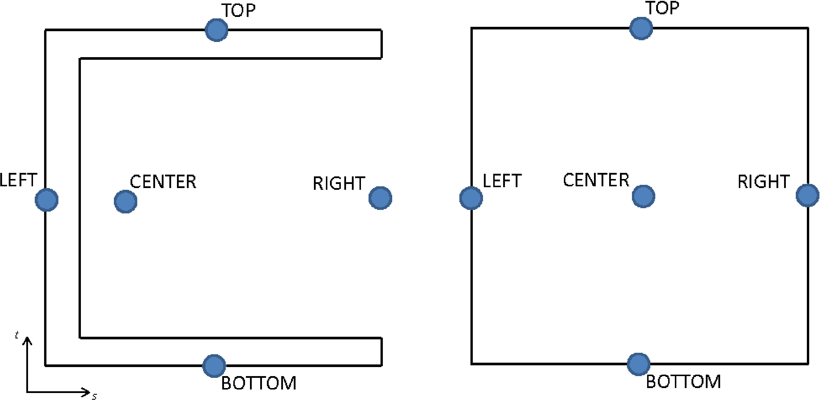
Fig. 6.22 Locations of REFERENCE AXIS command options.

The AXIS OFFSET command line allows the user to offset the local coordinate system from the geometric center line by an arbitrary distance. The s_offset value shifts the \(r\)-axis along the beam local \(s\)-axis. The t_offset value shifts the \(r\)-axis along the beam local \(t\)-axis. The \(s\), \(t\), and \(r\) axes are only shifted, not rotated by this offset.

Alternatively, the axis offset can be specified in global coordinates using the AXIS OFFSET GLOBAL command. This command takes three parameters, which are the \(x\), \(y\), and \(z\) components of the offset in the global coordinate system. Only the portion of the offset that lies in the element local \(s\) \(t\) plane will be used for the offset.

The AXIS OFFSET VARIABLE variable command behaves similar to the AXIS OFFSET command except that the offsets are specified element by element as defined by the input axis_offset_var field. This field should have two entries per element to define the element local \(s\) and \(t\) offsets.

6.2.8.2. Section Integration

Strains and stresses are computed at the midpoint of the two noded beam element beam. The integration of the stresses over the cross section at the midpoint is used to compute the internal forces in the beam. Each beam section has its own integration scheme.

The integration scheme for each of the sections is shown in Fig. 6.9 through Fig. 6.21. The numbers in these figures show the relative location of the integration points in the \(s\) \(t\) coordinate system.

Warning

Beam integration point shear stresses only account for torsional shear strains and do not contain effects due to transverse shear strains. Transverse shear forces are calculated from a linear elastic approximation using the given elastic constants and cross section. See the following discussion for more details.

At each integration point the beam element calculates strains and stresses that are related by the chosen material model. The formulation of the beam is like the typical Timoshenko theory and allows for transverse shear strains. However, in the Sierra/SM beam element the transverse shear is treated separately from the other strains. The axial stresses and strains are fully accounted for at the integration points, but the shear strains at the integration points are due only to the torsional deformation. In addition, the shear stress at the integration points is the circumferential torsional shear stress, with respect to the \(r\) axis, and the radial torsional shear stress is assumed to be zero (accurate for circular cross sections, an approximation for others). The transverse shear response is considered to be linear elastic, and the transverse shear contribution to the internal forces and moments is added apart from the contributions from the integration over the cross section. The linear elastic response is based on the user specified elastic constants.

Users should exercise caution when using the beam element with plasticity in problems that have large deformations or thick beams. Since the transverse shear response is only linear elastic, it will not properly account for other material models. Also, users should be careful to account for the integration point shear stresses only containing circumferential torsional shear stress.

Integration point data can be output for beam elements in much the same manner that it is requested for other elements by using commands in the RESULTS OUTPUT command block as described in Section 9. At each integration point, there are two components of strain and two components of stress. These components of stress and strain are in the axial and in-plane circumferential directions. The integration-point strain variables are named beam_strain_axial and beam_strain_shear, and the integration-point stress variables are beam_stress_axial and beam_stress_shear. In addition, state data is available at each integration point.

An important aspect of integration point output for beam elements is that the data is output in arrays sized by the number of integration points for the chosen beam cross-section (for example 9 for a rod and 15 for an I).

The beam axial and shear strains and stresses are output in sequence with the integration point numbering. For example, the first value of beam_strain_axial, designated in the output as _1 for a rod or _01 for the other sections, is the axial strain at the first integration point. The numbering continues to the number of integration points for that beam section – up to _9 for rod sections, _15 for I sections, and _16 for other sections.

An alternative method of accessing the stress is through the symmetric tensor unrotated_stress. Because a beam element uses local axes (i.e., a co-rotational system), unrotated_stress is given with respect to the \(r\), \(s\), and \(t\) coordinate system, and its _xx and _xy components are equivalent to the axial and torsional circumferential shear stresses, respectively, discussed above. Stress in general is stored as a symmetric tensor that contains six components, but for beams four of these components are never used. The axial stress at the first integration point is designated by unrotated_stress_xx_01 (or unrotated_stress_xx_1 for a rod section, with this pattern true for all integration point quantities discussed below) and the circumferential torsional shear stress at the first integration point is unrotated_stress_xy_01. The other four components, unrotated_stress_yy_01, unrotated_stress_zz_01, unrotated_stress_yz_01 and unrotated_stress_xz_01, are unused and are set to zero. The stresses at other integration points are named unrotated_stress_xx_NN and unrotated_stress_xy_NN, where NN is a number from 01 to 16.

Optionally the lofted geometry and a visual representation of beam integration point locations may be included in the output mesh file with use of the VISUALIZE INTEGRATION POINTS = ON command. When the extra visualization is turned on each beam will be represented both by the original line element and also and by a set of brick elements. The brick elements will represent the shape of the beam cross section, there will be one brick element per beam integration point. The visualize integration points option can be helpful in ensuring that the beam is being setup as desired both in size, orientation, and offsets from the neutral axis.

When using the VISUALIZE INTEGRATION POINTS command some beam integration point quantities can be visualized directly on the lofted hexahedral geometry. Any field that is defined at beam integration points will be copied out to the hexahedral representation elements. For example this includes fields such as:

• intg_point: Integration point number

• intg_weight: Integration point weight, should sum to 1.0 over all the integration points.

• intg_shear_flow_dir: Integration point shear flow direction

• beam_stress_axial: Axial component of beam stress

• beam_stress_shear: Shear component of beam stress

• beam_strain_axial: Axial component of beam strain

• beam_strain_shear: Shear component of beam strain

• lame_state_<model_name>: Material state variables.

It is possible to access mean values for the internal forces at the midpoint of the beam. The axial force at the midpoint of the beam is obtained by referencing the variable beam_axial_force. The transverse forces at the midpoint of the beam in the \(s\)-direction and the \(t\)-direction are obtained by referencing beam_transverse_force_s and beam_transverse_force_t, respectively. The torsion at the midpoint of the beam (the moment about the \(r\)-axis), is obtained by referencing beam_moment_r. The moments about the \(s\)-axis and the \(t\)-axis are obtained by referencing beam_moment_s and beam_moment_t, respectively.

Elements in a section can be made rigid by including the RIGID BODY command line. The RIGID BODY command line specifies an identifier that maps to a rigid body command block. See Section 6.3.1 for a full discussion of how to create rigid bodies and Section 6.3.1.1 for information on the use of the RIGID BODIES FROM ATTRIBUTES command.

Under certain conditions, the rotational mass of beams will be automatically scaled. This scaling is performed only when the computed time step from the axial modes is larger than the computed time step using the bending modes. This allows for larger critical time steps to be taken during the simulation. However, the user does have the option to turn it OFF via the ROTATIONAL MASS SCALING line command.

6.2.8.3. Beam Element Accuracy

It is worth noting that due to a finite accuracy integration rule the integration error in beam behavior is dependent on the loading case. For pure axial loading, the error is nearly zero throughout both the elastic and plastic regimes for all cross sections. This is due to axial resistance being a function of sectional area, which is explicitly computed from section properties.

However, in the bending cases there is varying levels in error dependent on section, bending direction, and loading value. In general, the error percentage is low (roughly 1 to 2%) for very elastic loadings in the \(s\)- and \(t\)- bending directions when strain is about \(10^{-6}\). Thin-walled sections with more integration points, such as the hat, are more accurate in bending in both the elastic and plastic regimes when bent in the \(s\)- and \(t\)-directions. Error can be larger (up to 10%) for elastic bending in directions of than the \(s\) and \(t\) axis. Additionally errors will tend to be larger (up to 10%) in the elastic plastic or fully plastic transition regimes.

Torsional loading for some cross sections can potentially produce large error. The integration assumes no out of plane warping during torsion. Thus the torsional resistance of sections that do have out of plane warping (open sections) may be greatly over estimated. For example, the circular rod will see no sectional warping thus having less deviation from the analytical solution, particularly in the elastic regime. However, the hat cross section would see high amounts of sectional warping which is not fully accounted for in the solution produced by the code. In cases such as this, results will be vastly different than their analytical solutions. Additionally, it is important to point out that there is no bend-twist twist coupling for open sections, as this produces spurious unstable behavior.

6.2.9. Truss Section

BEGIN TRUSS SECTION <string>truss_section_name
  AREA = <real>cross_sectional_area
  DIAMETER = <real>diameter
  AREA MESH VARIABLE = <string>area_var_name
  INITIAL LOAD = <real>initial_load
  PERIOD = <real>period
  RIGID BODY = <string>rigid_body_name
  RIGID BODIES FROM ATTRIBUTES = <integer>first_id
    TO <integer>last_id
END [TRUSS SECTION <string>truss_section_name]

The TRUSS SECTION command block specifies the properties for a truss element. If this command block is referenced in an element block of three-dimensional, two-node elements, the elements in the block will be treated as truss elements. The parameter, truss_section_name, is user-defined and is referenced by a SECTION command line in a PARAMETERS FOR BLOCK command block.

The cross-sectional area for truss elements can specified by the AREA command line. Alternatively the area can be set by defining the diameter for the cylindrical truss element. If specified the value cross_sectional_area or diameter will be used for all truss elements of the block element block. Alternatively the AREA MESH VARIABLE may be used to provide the name of a variable on the input genesis mesh that lists the element by element attributes. If the truss area is provided by an element attribute, the area_var_name should be set to “attribute.” Note one and only one of AREA, DIAMETER, or AREA MESH VARIABLE must be given for the truss section.

The truss can be given some initial load over some given time period. The magnitude of the load is specified by the INITIAL LOAD command line. If the load is compressive, the sign on the value initial_load should be negative; if the load is tensile, the sign on the value initial_value should be positive. The period is specified by the PERIOD command line.

The initial load is applied over some period by specifying the axial strain rate in the truss, \(\dot{\varepsilon}\), over some period \(p\). At some given time \(t\), the strain rate is

(6.3)\[\dot \varepsilon = \frac{{ap}}{2}\left[ {1 - \cos \left(\pi t/p\right)} \right],\]

where

(6.4)\[a = \frac{{2F_i }}{{EAp}}.\]

In (6.4), \(F_{i}\) is the initial load, \(E\) is the modulus of elasticity for the truss, and \(A\) is the area of the truss. Over the period \(p\), the total strain increment generates the desired initial load in the truss.

During the initial load period, the time increments should be reasonably small so that the integration of \(\dot{\varepsilon}\) over the period is accurate. The period should be set long enough so that if the model was held in a steady state after time \(p\), there would only be a small amount of oscillation in the load in the truss.

Certain boundary conditions should not be activated until after the pre-stressing is done. During the pre-stressing, time-independent boundary conditions such as fixed displacement will most likely be turned on. Time-dependent boundary conditions such as prescribed acceleration or prescribed force will most likely be activated after the pre-stressing is complete.

Elements in a section can be made rigid by including the RIGID BODY command line. The RIGID BODY command line specifies an indenter that maps to a rigid body command block. See Section 6.3.1 for a full discussion of how to create rigid bodies and Section 6.3.1.1 for information on the use of the RIGID BODIES FROM ATTRIBUTES command.

Warning

Truss elements currently do not work correctly as a rigid body due to lack of cross-section geometry to define the moment of inertia about the truss axis. They should be used only if the user explicitly includes the command line INERTIA = in the RIGID BODY command block to specify the mass moment of inertia for the entire rigid body. (See Section 6.3.1.) The recommendation is to use beam elements for rigid bodies rather than truss elements if possible.

Axial stress, which is the only stress component for a truss element, is output as a symmetric tensor with six components to be compatible with the notion of volumetric stress. Because of this, for every truss element, six values of stress are stored and output, but only the fist value is ever used. The axial stress is therefore output as stress_xx and the other five stress components, stress_yy, stress_zz, stress_xy, stress_yz, stress_zx are all unused and set to zero.

6.2.10. Spring Section

BEGIN SPRING SECTION <string>spring_section_name
  FORCE STRAIN FUNCTION = <string>force_strain_function
  DEFAULT STIFFNESS <real>default_stiffness
  PRELOAD = <real>preload_value
  PRELOAD DURATION = <real>preload_duration
  RESET INITIAL LENGTH AFTER PRELOAD = <string>NO|YES
  MASS PER UNIT LENGTH = <real>mass_per_unit_length
END [SPRING SECTION <string>spring_section_name]

The SPRING SECTION command block specifies the properties for a spring element. If this command block is referenced in an element block of three-dimensional, two node elements, the elements in the block will be treated as spring elements. The parameter, spring_section_name, is user-defined and is referenced by a SECTION command line in a PARAMETERS FOR BLOCK command block.

The spring behavior is governed by the force-engineering strain function which is specified by the FORCE STRAIN FUNCTION command line. The force generated by the spring element is based on the evaluation of the user specified force_strain_function, which has units of force. The strain is defined by \((L_i-L_0)/L_0\) with \(L_i\) the current spring length and \(L_0\) the original spring length. This allows the force-strain function to be length independent.

Positive values of the force strain function correspond to tension and negative values to compression. The force-strain function should be defined over the full range of strains that the spring may see, both positive and negative. The following are examples of possible spring stiffness functions.

BEGIN FUNCTION FORCE_STRAIN_2
  # "x" is the signed input strain value
  # This is a linear spring with stiffness of 1000
  TYPE = ANALYTIC
  EVALUATE EXPRESSION = "1000*x"
END

BEGIN FUNCTION FORCE_STRAIN_3
  # Nonlinear "chain" element. Has stiffness in tension only
  TYPE = PIECEWISE LINEAR
  BEGIN VALUES
     0     0
     5  5000
  END
END

BEGIN FUNCTION FORCE_STRAIN_1
  # Nonlinear complex spring with gaps and variable stiffness
  TYPE = PIECEWISE LINEAR
  BEGIN VALUES
    -0.5 -1000
    -0.1     0
     0       0
     0.1  1000
     0.2  5000
     0.5 10000
  END
END

The DEFAULT STIFFNESS command block specifies the spring stiffness used during the first time step and during preload. In all other situations the spring stiffness is based on the slope of the force-strain function evaluated at the previous time step and the current time step. The unit of default_stiffness is force.

To specify a preload on the spring both the PRELOAD and PRELOAD DURATION command line must be specified. The PRELOAD command line specifies the magnitude of the preload force, while the PRELOAD DURATION command line specifies how long the preload application should take, in seconds. The preload force will be initially set to 0 and ramp up to the PRELOAD value when your simulation reaches 95% of the PRELOAD DURATION. After reaching 95%, the preload will remain constant.

An optional preload input, RESET INITIAL LENGTH AFTER PRELOAD, is used when the user would like the initial length of the spring to reset to the displaced length after the preload has occurred. If this command line is not specified, or is set to NO, the initial length of the spring is the undeformed length as calculated from the input mesh.

Springs can have a mass as defined by the MASS PER UNIT LENGTH command line. When defining the spring section this value must be specified. A zero mass spring is allowed by setting MASS PER UNIT LENGTH explicitly to zero. Note, in explicit computations if the spring has no mass the spring has no defined element time step. For a mass-less spring the effect of the spring on the global time step will be factored into the nodal Section 3.2.3.1 or Lanczos Section 3.2.1.5 time step estimates.

6.2.11. Damper Section

BEGIN DAMPER SECTION <string>damper_section_name
  AREA = <real>damper_cross_sectional_area
  VISCOSITY COEFFICIENT FUNCTION = <string>function_name (optional)
END [DAMPER SECTION <string>damper_section_name]

The DAMPER SECTION command block specifies the properties for a damper element. If this command block is referenced in an element block of three-dimensional, two-node elements, the elements in the block will be treated as damper elements. The parameter, damper_section_name, is user-defined and is referenced by a SECTION command line in a PARAMETERS FOR BLOCK command block.

The cross-sectional area for damper elements is specified by the DAMPER AREA command line. The value damper_cross_sectional_area is the cross-sectional area of the dampers in the element block.

The damper area is used only to generate mass associated with the damper element. The mass is the density for the damper element multiplied by the original volume of the element (original length multiplied by the damper area).

The force generated by the damper element depends on the relative velocity along the current direction vector for the damper element. If \(\mathbf{n}\) is a unit normal pointing in the direction from node 1 to node 2, if \(\mathbf{v}_1\) and \(\mathbf{v}_2\) are the velocity vectors at nodes 1 and 2, respectively, then the force generated by the damper element is

(6.5)\[F_d = \eta(v_{rel})v_{rel}\quad\text{where}\quad v_{rel} = \mathbf{n} \cdot \left( \mathbf{v}_2 - \mathbf{v}_1 \right).\]

The damping viscosity coefficient \(\eta(v_{rel})\) may be a constant value, or specified as a function of the relative velocity \(v_{rel}\). To specify a constant value, the damper section will extract the value for Young’s modulus in the elastic material model used for the element block assigned the damper section.

Alternatively, a damping function may be specified using the VISCOSITY COEFFICIENT FUNCTION. The function assigned by VISCOSITY COEFFICIENT FUNCTION refers to a SIERRA function and is evaluated as a function of the relative velocity \(v_{rel}\). Specifying a constant function here is equivalent to specifying a constant value via the material Young’s modulus.

For stability purposes, the viscosity coefficient should be positive for all values of \(v_{rel}\).

Warning

The damper section does not provide a critical time step estimate. However, including a damper can impact stability by reducing stable time step when attached to a large model. It may be necessary to manually reduce the explicit time step using the TIME STEP SCALE FACTOR line command if stability issues arise.

6.2.12. Point Mass Section

BEGIN POINT MASS SECTION <string>pointmass_section_name
  VOLUME = <real>volume
  MASS = <real>mass
  IXX = <real>Ixx
  IYY = <real>Iyy
  IZZ = <real>Izz
  IXY = <real>Ixy
  IXZ = <real>Ixz
  IYZ = <real>Iyz
  RIGID BODY = <string>rigid_body_name
  RIGID BODIES FROM ATTRIBUTES = <integer>first_id
    TO <integer>last_id
  MASS VARIABLE = <string>mass_variable_name
  INERTIA VARIABLE = <string>inertia_variable_name
  OFFSET VARIABLE = <string>offset_variable_name
  ATTRIBUTES VARIABLE NAME = <string>attrib_variable_name
END [POINT MASS SECTION <string>pointmass_section_name]

A point mass element is a mass at a node, which can be a convenient modeling tool in certain instances. The user can create an element block with one or more point masses. A point mass is a sphere element attached to a single node. A point mass will have its mass added to the mass at the connected node. (Other mass at the node will be derived from mass due to elements attached to the node.) The mass at a node due to a point mass is treated like any other mass at a node derived from an element. The mass due to point mass will be included in body force calculations and kinetic energy calculations, for example.

Point masses are a convenient modeling tool to be used in conjunction with rigid bodies. An element block including one or more point masses can be included in a collection of element blocks used to define a rigid body. The element block of point masses can be used to adjust the total mass and inertia properties for the rigid body. (The point mass element does not have to be used only in conjunction with rigid bodies. One can place a point mass at a node associated with solid or structural elements.)

An element block in which the connectivity for each element contains only one node can be used as a collection of point masses. This command block would have the following form:

BEGIN PARAMETERS FOR BLOCK <string>block_id
  MATERIAL = <string>material_name
  MODEL    = <string> material_model_name
  SECTION = <string>point_mass_section_name
END PARAMETERS FOR BLOCK <string>block_id

The element block associated with the point mass must reference a material command block just like any other element block. If the point mass section specifies a volume, then the product of the density specified in the material block and the volume specified in the section block is used to calculate the element mass.

The VOLUME command specifies the volume of a point mass element. The mass of the element is then found by multiplying that volume by the material model density.

The MASS command explicitly specifies the mass.

The IXX, IYY, IZZ, IXY, IXZ, IYZ commands are used to explicitly define the symmetric inertia tensor entries for the point mass. Note that currently, the trace of the inertial tensor is added to the nodal rotational mass and the rest of the inertia tensor entries are ignored.

The OFFSET is used to define the offset of the mass with respect to the connected node. Currently the offset affects only the rotational properties of the point mass. The rotational mass of the point mass is increased by mass times offset distance squared.

The MASS VARIABLE specifies that the mass of the point mass elements is to be read from the input mesh file from the variable with the specified name (use the name “attribute” to read the mass from the mesh block attributes.)

The INERTIA VARIABLE specifies that the inertia tensor of the point mass elements is to be read from the input mesh file from the variable with the specified name (use the name “attribute” to read the inertia tensor from the mesh block attributes.) When this command is used, the mesh file variable should contain six entries per element, ordered as follows: Ixx, Iyy, Izz, Ixy, Ixz, and Iyz.

The OFFSET VARIABLE specifies that the offset vector of the point mass elements is to be read from the input mesh file from the variable with the specified name (use the name “attribute” to read the offset vector from the mesh block attributes.) When this command is used, the mesh file variable should contain three entries per element, ordered as follows: Offset_x, Offset_y, and Offset_z.

The ATTRIBUTES VARIABLE NAME specifies that all properties of the point mass element are to be read from the input mesh file of the variable with the specified name (use the name “attribute” to read from the mesh block attributes.) When this command is used, the mesh file variable should contain ten entries per element, ordered as follows: Mass, Ixx, Iyy, Izz, Ixy, Ixz, Iyz, Offset_x, Offset_y, and Offset_z.

Multiple ways are provided to specify the raw attributes of mass, inertia and offset for the point mass element. The user must be careful to only use one of these ways to define each property. Using multiple ways to define the mass will result in errors or warnings because of ambiguities.

If the user has access to the SEACAS codes from Sandia National Laboratories, The codes in this library may be used to generate element blocks with point mass elements. See Reference [[11]] for an overview of the SEACAS codes. By using various SEACAS codes, an element block with one or more point masses may be generated. For each point mass in the element block, an eight-noded hexahedral element centered at the point mass location should be created. The hexahedron may have arbitrary dimensions, but it is best to work with a unit cube. For example, to generate a point mass at coordinates (13.5, 27.0, 3.1415), a \(1 \times 1 \times 1\) (unit) hexahedron centered at (13.5, 27.0, 3.1415) should be created. The SEACAS program SPHGEN3D may be used to convert the hexahedron to a zero-dimensional element located at the center of the hexahedron in three-dimensional space. In the provided example, SPHGEN3D would create a zero-dimensional, single-noded element at coordinates (13.5, 27.0, 3.1415).

Elements in a section can be made rigid by including the RIGID BODY command line. The RIGID BODY command line specifies an indenter that maps to a rigid body command block. See Section 6.3.1 for a full discussion of how to create rigid bodies and Section 6.3.1.1 for information on the use of the RIGID BODIES FROM ATTRIBUTES command.

6.2.13. Particle Section

BEGIN PARTICLE SECTION <string>particle_section_name
  RADIUS MESH VARIABLE = ATTRIBUTE|RADIUS
  SPHERE INITIAL RADIUS = <real>rad
  RADIUS TIME STEP = <string>time
  PROBLEM DIMENSION = <integer>1|2|3(3)
  CONSTANT SPHERE RADIUS
  FINAL RADIUS MULTIPLICATION FACTOR = <real>factor(1.0)
  FORMULATION = <string>MASS_PARTICLE|SPH(SPH)
  MONAGHAN EPSILON = <real>monaghan_epsilon(0.0)
  MONAGHAN N = <real>monaghan_n(0.0)
  SPH ALPHAQ PARAMETER = <real>alpha(1.0)
  SPH BETAQ PARAMETER = <real>beta(2.0)
  DENSITY FORMULATION = <string>MATERIAL|KERNEL(MATERIAL)
  MAXIMUM RADIUS CHANGE = <real>minVal <real>maxVal
END [PARTICLE SECTION <string>particle_section_name]

SPH (smoothed particle hydrodynamics) is useful for modeling fluids or for modeling materials that undergo extremely large distortions. One must be careful when using SPH for modeling. SPH tends to exhibit both accuracy and stability problems, particularly in tension. An SPH particle interacts with other nearest-neighbor SPH particles based on radius properties of all the elements involved; SPH particles react with other elements, such as tetrahedra, hexahedra, and shells, through contact. Many more details on the theoretical background of SPH are available in [[12]].

Contact interactions between the particles in a particle element block and other element types may be defined using the CONTACT NODE SET option described in Section 8.4.2. All particles in the particle element block must be included in a node set if the CONTACT NODE SET option is used.

The particle section should only be associated with elements with the SPHERE topology. Sphere elements are point elements that are connected to only a single node.

All the particles contained in a particle element block must be given some initial radius. There are two options for setting the initial radius for each particle. First, each particle can be given the same radius. To set the radius for each particle in an element block to the same value, use the SPHERE INITIAL RADIUS command line. The parameter rad on this command line sets the radius for all the particles in the element block.

Alternatively, the radius for each particle can be read from a mesh file. The radii can be read from a variable on the mesh file from attributes associated with the element block. To read some variable from the mesh file for the radii, the command

RADIUS MESH VARIABLE = RADIUS

may be used, where radius is the variable name on the mesh file. To use the variable associated with a specific time on the mesh file, the RADIUS TIME STEP command line should be used to select the specific time. To read the attributes associated with the particles, the command line

RADIUS MESH VARIABLE = ATTRIBUTE

should be inserted (as shown) into the PARTICLE SECTION command block. Pronto3D [[13]] only offers the attribute option. The attribute option should be used to compare Sierra/SM and Pronto3D results.

If the attribute option is used, each particle should have two attributes defined per element. The first attribute is the particle radius, and the second attribute is the particle volume. The most common way to generate a particle mesh is to first generate a solid element mesh and then use the utility ‘sphgen3d’ to convert the solid elements into sphere elements. Sphgen3d will convert each solid element into a sphere and place it at the source element centroid. In the output mesh file generated by sphgen3d The radius attribute of the element blocks will be proportional to the source element size and the volume attribute will be the volume of the source element.

The FINAL RADIUS MULTIPLICATION FACTOR command may be used to increase or decrease the initial particle radii. The factor specified will scale the particle radii input with either a constant or a mesh file attribute.

After the radii are initialized, the user may specify whether the radii are to remain constant or are to change throughout the analysis. The CONSTANT SPHERE RADIUS command line is an optional command line that prevents the sphere radius from changing over the course of the calculation. By default, the sphere radii will expand or contract based on the changing density in the elements to satisfy the relation that element mass (a constant) equals element volume times element density. If the CONSTANT SPHERE RADIUS command line appears, then the radii for all particles will remain constant.

The DENSITY FORMULATION command controls the method used to update the density, and thus SPH radii, during the analysis. The default MATERIAL option uses the material density and nodal mass to compute a volume for each particle at a given time. The radius is then computed as the cube root of that volume. The alternative KERNEL option computes the current density for each particle using the mass of that particle and the SPH kernel density function. The KERNEL option may be necessary when large expansions of particles are expected (such as when modeling large density changes in gases). The MATERIAL option generally changes particle densities, and thus radii, less than the KERNEL option, so is appropriate for analyses that do not have large density fluctuations.

The MAXIMUM RADIUS CHANGE command may be used to control how much a given SPH particle is allowed to expand or shrink over the course of the analysis. For example, setting

MAXIMUM RADIUS CHANGE = 0.2 10.0

would indicate that the radius of any particle cannot become less than 20% or more than 1000% of the particle’s original radius. By default, the particle can shrink or expand as much as its density change requires. This option may be useful, for example, in explosive modeling if the particle radii are expanding excessively causing analysis performance and stability problems.

An analysis using SPH may be inherently one-, two-, or three-dimensional. Dimensionality of the problem may be specified using the PROBLEM DIMENSION command line. The possible value for this command line is 1 (one-dimensional), 2 (two-dimensional), or 3 (three-dimensional). The default value is 3 for three-dimensional. The internal SPH kernel functions are modified depending on the value set on the PROBLEM DIMENSION command line. If, for example, a problem is inherently two-dimensional in nature, more accurate results may be obtained by specifying the dimension of the problem as 2.

The FORMULATION command defines the SPH formulation to use, and has the following options:

• SPH, general smoothed particle hydrodynamics.

• MASS_PARTICLE, Particles only have mass, and no stiffness. Particles do not interact with each other in any way.

The MONAGHAN EPSILON and MONAGHAN N commands set the Monaghan viscosity coefficients. Monaghan viscosity may allow the SPH algorithm to behave better, particularly in tension. Standard values to use are 0.2 for epsilon and 4 for n. See (Reference [[14]]) for more information on the usage of these parameters.

The SPH ALPHAQ PARAMETER and SPH BETAQ PARAMETER commands control the SPH viscosity terms. Larger values lead to more viscosity. Alpha is associated with a viscosity parameter that is proportional to the dilatational modulus of the material. Betaq is associated with a viscosity parameter that is proportional to the change in material density over a time step.

Utility commands. In addition to the SPH-related command lines described above (which appear in the PARTICLE SECTION command block), the BEGIN SPH OPTIONS is another SPH-related command block:

BEGIN SPH OPTIONS
  SPH SYMMETRY PLANE <string>+X|+Y|+Z|-X|-Y|-Z
    <real>position_on_axis(0.0)
  SPH DECOUPLE STRAINS: <string>material1 <string>material2
END [SPH OPTIONS]

If used, this command block should be placed in the Presto region scope (in contrast to most SPH-related commands which are in the PARTICLE SECTION command block). The symmetry conditions are applied to all SPH element blocks.

The SPH SYMMETRY PLANE command line may be used to reduce model sizes by specifying symmetry planes and modeling only a portion of the model. Due to the non local nature of SPH element integration, symmetry planes cannot be defined with boundary conditions alone; these planes must be explicitly defined. A plane is defined by an outward normal vector aligned with one of the axes (+X, +Y, +Z, -X, -Y, -Z) and some point on the axis, which represents a point in the plane. Suppose for example, the outward normal to the plane of symmetry is in the negative \(Y\)-direction (-Y) and the plane of symmetry passes through the \(y\)-axis at \(y = + 2.56\). Then the definition for the symmetry plane would be:

SPH SYMMETRY PLANE -Y +2.56

The SPH DECOUPLE STRAINS command line prevents two dissimilar materials from directly interacting. Generally, the material properties at a particle are the average of the material properties from nearby particles. If particles with very dissimilar material properties are interacting, this interaction can create problems. The SPH DECOUPLE STRAINS command line ensures that particles with very dissimilar material properties do not directly interact by material-property averaging, but instead interact with a contact-like interaction. The two material types that are not to interact are specified by the parameters material1 and material2. These parameters will appear as material names on a MATERIAL command block.

Conversion to particles at initialization. To facilitate the creation of particle-based meshes, an additional SPH-related command block is the BEGIN CONVERSION TO PARTICLES AT INITIALIZATION block:

BEGIN CONVERSION TO PARTICLES AT INITIALIZATION
  BLOCK = <string list>block_names
  SECTION = <string>particle_section
END [CONVERSION TO PARTICLES AT INITIALIZATION]

This block, which must be placed in the Presto region scope, specifies that an input mesh consisting of solid elements be converted into particles at initialization. Particle elements are created at the centroid of each element with appropriate mass and volume, and the initial solid elements of the input mesh are deleted. Any initial and boundary conditions are inherited from the corresponding initial solid element; furthermore, the particle will be associated with the same node set or side set which any node of the parent element belongs to.

Only elements within the blocks specified by the BLOCK command will be converted to particles. Each new element will be assigned an arbitrary, but new and unique global numerical ID.

The SECTION command must specify a user-defined section of SPH type; it is important to note that the SECTION command originally associated with the initial solid element-block command block(s) will therefore be disregarded. It is worth noting that a particle section should not be specified in the initial solid element-block command block(s), since particle sections are not compatible with solid element input mesh topologies; instead, a compatible solid element section should be specified in the initial element-block definition(s).

Display. For purposes of visualizing the element stresses, it may be necessary to copy these element variables into nodal variables. This can easily be done by defining a USER VARIABLE command block (Section 10.2.4) in conjunction with a USER OUTPUT command block (Section 9.4). Once the nodal variable is defined, it can be output in a RESULTS OUTPUT command block (Section 9.3.1). An example is provided below. The SPH element blocks for the problem are element blocks 20, 21, and 22. All other element blocks are non-SPH elements.

• In the region scope:

  # Define the variable
  BEGIN USER VARIABLE nodal_stress
    TYPE = NODE SYM_TENSOR LENGTH = 1
  END
  #
  # Copy element stress to nodal stress
  BEGIN USER OUTPUT
    BLOCK = block_20 block_21 block_22
    COPY ELEMENT VARIABLE stress TO NODAL VARIABLE nodal_stress
  END
  # Output nodal stress
  BEGIN RESULTS OUTPUT output_presto
    DATABASE NAME = sph.e
    DATABASE TYPE = exodusII
    AT TIME 0.0 INCREMENT = 1.0e-04
    NODAL nodal_stress
  END RESULTS OUTPUT output_presto
  

Known Issue

For problems with rotations, the SPH algorithm generates rotational spring like forces on the boundary because of known deficiencies in the algorithm in distinguishing between rigid body rotation and deformation. The SPH algorithm does not conserve rotational or angular momentum.

Known Issue

If a BEGIN PRESSURE (Section 7.7.1) block is used with the CONVERSION TO PARTICLES AT INITIALIZATION command, the pressure is not applied. Pressure can be applied to particles by using the ELEMENT DEATH command block (Section 6.5).

6.2.14. Superelement Section

BEGIN SUPERELEMENT SECTION <string>section_name
   BEGIN MAP
     <integer>node_index_1 <integer>component_index_1
     <integer>node_index_2 <integer>component_index_2
     ...
     <integer>node_index_n <integer>component_index_n
   END
   BEGIN STIFFNESS MATRIX
     <real>k_1_1 <real>k_1_2 ... <real>k_1_n
     <real>k_2_1 <real>k_2_2 ... <real>k_2_n
     ...         ...         ... ...
     <real>k_n_1 <real>k_n_2 ... <real>k_n_n
   END
   BEGIN DAMPING MATRIX
     <real>c_1_1 <real>c_1_2 ... <real>c_1_n
     <real>c_2_1 <real>c_2_2 ... <real>c_2_n
     ...         ...         ... ...
     <real>c_n_1 <real>c_n_2 ... <real>c_n_n
   END
   BEGIN MASS MATRIX
     <real>m_1_1 <real>m_1_2 ... <real>m_1_n
     <real>m_2_1 <real>m_2_2 ... <real>m_2_n
     ...          ...        ... ...
     <real>m_n_1 <real>m_n_2 ... <real>m_n_n
   END
   FILE = <string>netcdf_file_name
   CONNECTIVITY MAPPING =
                  BY GLOBAL NODE PROXIMITY <real>dist
   CONNECTIVITY MAPPING = BY GLOBAL NODE ID
   DIAGONALIZE MASS MATRIX = OFF|ON (OFF)
   COROTATION FORMULATION = OFF|ON (OFF)
END [SUPERELEMENT SECTION <string>section_name]

A superelement allows definition of an arbitrary sized connectivity element with full stiffness, damping, and mass matrices. The superelement stiffness is linear and remains constant in time.

Known Issue

Superelements are not compatible with several modeling capabilities:

• They cannot be used with

  • contact,

  • element death,

  • node-based, power method, or Lanczos critical time step estimation

    methods, and

  • some preconditioners (such as FETI) for implicit solutions.

• Superelements are not fully tested with restart.

6.2.14.1. Defining a Superelement

A superelement may be defined either (i) in a separate NetCDF file or (ii) directly in the input deck.

A superelement may be defined in an input file using the FILE option. This command expects a NetCDF file generated by the Salinas Craig-Bampton reduction capability. The Salinas output file contains superelement mass, damping, and stiffness matrices, as well as locations and nodal IDs of the superelement interface nodes. When defining a superelement from an input file, the element block used to define the superelement should be excluded from the Sierra/SM analysis input mesh; instead, the superelement input file will fully define this block.

Superelement interface nodes can be merged onto Sierra/SM model nodes to make a contiguous link. The default method to merge superelement interface nodes onto the rest of the mesh is to merge nodes with the same nodal ID using the command

CONNECTIVITY MAPPING = BY GLOBAL NODE ID

Alternatively, spatially coincident nodes may be merged with the command

CONNECTIVITY MAPPING = BY GLOBAL NODE PROXIMITY

When using proximity mapping, an absolute search distance may be given to merge nearby nodes. Any superelement interface node not merged on to a mesh node will be created on the fly and given an ID number and location as defined by the NetCDF file.

A superelement may also be defined directly in the input deck. When using this method, each component of the superelement mass, damping, and stiffness matrices must be specified. The superelement itself must also be represented by an element in the input mesh file. The block of elements used to define a superelement must contain exactly one finite element of arbitrary topology of the user’s choosing, e.g., a valid geometric topology (hexahedral, rod, tetrahedral, etc.). The nodes of a superelement can be shared with other elements or attached only to the superelement. The superelement can have additional internal degrees of freedom that are not present in the mesh file. However, if output values are desired on a node, that node must be present in the input mesh file.

• The MAP command block defines the mapping from nodal degrees of freedom to the local degrees of freedom in the stiffness and mass matrices for the superelement. If the superelement is defined using the FILE command, this mapping information is contained in that file and need not be specified in the input deck.

  If defined, the map is of size \(M \times 2\), where \(M\) is the number of degrees of freedom in the superelement. The first column contains each index \(i_{nod}\) of the node in the superelement, \(0 \le i_{nod} \le N\), where \(N\) is the number of nodes in the superelement, while the second column contains the component corresponding to each superelement degree of freedom \(j_{comp}\), \(0 \le j_{comp} \le 6\).

  Any \(i_{nod} = 0\) indicates a degree of freedom internal to the superelement. A superelement may have any number of internal degrees of freedom which need not correspond to any nodes actually present in the mesh. Any \(i_{nod} > 0\) represents the corresponding node index in the element. For example, a superelement consisting of an eight-node hexahedral element would have \(N = 8\) and \(1 \le i_{nod} \le 8\) corresponding to each node in the hexahedron.

  Component indices \(j_{comp} = 0\) represent internal degrees of freedom, while \(1 \le j_{comp} \le 6\) indicate physical components on nodes in the mesh; for a standard node, component indices 1, 2, and 3 correspond to \(x\), \(y\), and \(z\) translational degrees of freedom. Components 4, 5, and 6 correspond to the \(x\), \(y\), and \(z\) rotational degrees of freedom for structural elements.

  The following is an example superelement definition for a three-degree-of-freedom truss element lying along the \(x\)-axis. The superelement is defined in the mesh file using a two-node rod element. Degrees of freedom 1 and 3 are mapped to \(x\) degrees of freedom of the end nodes of the rod element. Degree of freedom 2 is internal to the superelement.

  BEGIN SUPERELEMENT SECTION truss_x3
    BEGIN MAP
      1 1
      0 0
      2 1
    END
    BEGIN STIFFNESS MATRIX
      100 -100    0
     -100  200 -100
        0 -100  100
    END
    BEGIN DAMPING MATRIX
      1 -1  0
     -1  2 -1
      0 -1  1
    END
    BEGIN MASS MATRIX
      0.25 0.00 0.00
      0.00 0.50 0.00
      0.00 0.00 0.025
    END
  END [SUPERELEMENT SECTION <string>section_name]
  

• The STIFFNESS MATRIX command block defines the \(N \times N\) stiffness matrix for the superelement. If the superelement is defined using the FILE command, this stiffness information is contained in that file and need not be specified in the input deck. The number of rows and columns in the stiffness matrix must be the same as the number of rows in the MAP command block. The stiffness matrix should be symmetric. If the input matrix is not symmetric, it will be made symmetric by \(K_{sym} = \tfrac{1}{2}(K_{input} + K_{input}^T)\). To guarantee stability for explicit dynamics and solution convergence for implicit statics/dynamics, the stiffness matrix should be positive definite.

• The DAMPING MATRIX command block defines the \(N \times N\) damping matrix for the superelement. If the superelement is defined using the FILE command, this damping information is contained in that file and need not be specified in the input deck. The number of rows and columns in the damping matrix must be the same as the number of rows in the MAP command block. The damping matrix should generally be symmetric. This command block is optional. If a damping matrix is not defined, no damping will be used by default.

• The MASS MATRIX command block defines the \(N \times N\) mass matrix for the superelement. If the superelement is defined using the FILE command, this mass information is contained in that file and need not be specified in the input deck. The mass matrix must have the same dimensions as the stiffness matrix. The mass matrix need not be symmetric; however, to guarantee stability for explicit dynamics and solution convergence for implicit statics/dynamics, the mass matrix should be positive definite.

• The FILE command provides an alternative to defining stiffness, damping, mass, and connectivity in the input file. Instead, this information can be imported from an external file. External codes (such as Salinas) are able to compress larger models into superelements and output the matrices in the NetCDF format. The netcdf_file_name defines the path to the file that contains the mass, damping, and stiffness matrix definitions as well as interface node locations and connectivity. All superelement matrices should be defined either in the input deck or in the NetCDF file. The damping matrix is optional; if it is not defined in the NetCDF file, no damping will be used by default. In the NetCDF file the stiffness matrix must be named Kr, the mass matrix Mr, and the damping matrix Cr.

• Superelements may have a full, consistent mass matrix. This consistent mass matrix is incompatible with some code capabilities such as contact, MPCs, or kinematic boundary conditions. The mass matrix may be optionally diagonalized via the DIAGONALIZE MASS MATRIX, enabling the superelement to be more compatible with some of these capabilities.

• The COROTATION FORMULATION command should be used when superelement connection nodes experience large rigid body rotations. The corotation formulation incorporates a rotation matrix to minimize the root mean square deviations between the model coordinates and the current coordinates of the superelement connection nodes into superelement computations.

6.2.14.2. Superelement Output Variables

Superelement nodes have the same variables as traditional nodes (mass, displacement, velocity, etc.). Only the element time step is defined as an output variable on the superelement itself.

6.2.14.3. Specifying Initial Conditions and Loads on Superelements

Superelements currently support constant initial velocities and gravity loads. Initial velocities and gravity loads on superelements are specified using special input syntax in the INITIAL VELOCITY and GRAVITY command blocks (consult Section 7.5 and Section 7.9 for general details).

Superelements only support constant initial velocities given by a magnitude and direction. To specify an initial unit velocity in the \(y\)-direction on all blocks in a given model, including superelement super_elem:

BEGIN INITIAL VELOCITY
  INCLUDE ALL BLOCKS
  SUPER ELEMENT = super_elem
  DIRECTION = Y
  MAGNITUDE = 1.
END

Superelements only support constant gravity loadings given by a gravitational constant and component direction. To specify a gravity loading in the \(y\)-direction on all blocks in a given model, including superelement super_elem:

BEGIN GRAVITY
  INCLUDE ALL BLOCKS
  SUPER ELEMENT = super_elem
  COMPONENT = Y
  GRAVITATIONAL CONSTANT = 386.1
  SCALE FACTOR = 1.
END

6.2.15. User Mount Section

BEGIN USER MOUNT SECTION <string>user_mount_section_name
  MOUNT TYPE = FAIL_TRUSS|SPRING_DASH_POT|SNUBBER|
     TORSIONAL_SPRING|6_DOF_LINEAR_SPRING|USER_SUBROUTINE
  PARAMETERS = <real list>data
  PARAMETERS VARIABLE = <string>attribute_name
  T AXIS = <real> <real> <real>
  T AXIS VARIABLE <string>attribute_name
  S AXIS = <real> <real> <real>
  S AXIS VARIABLE <string>attribute_name
  ZERO LENGTH R AXIS = <real> <real> <real>

  MOUNT FORCE SUBROUTINE = <string>mountForceSub
  MOUNT INIT  SUBROUTINE = <string>mountInitSub
  MOUNT SIZE  SUBROUTINE = <string>mountSizeSub
END [USER MOUNT SECTION <string>user_mount_section_name]

The USER MOUNT SECTION command block provides a capability to link two nodes with an arbitrary nonlinear connection. If this command block is referenced in an element block of three-dimensional, two node elements, the elements in the block will be treated as user mount elements. The name, user_mount_section_name, can be used by the SECTION command line in a PARAMETERS FOR BLOCK command block.

The MOUNT TYPE is command specifies a small number of USER MOUNT that have been implemented directly in the code rather than through user subroutines. Note that the user mounts were originally developed for use in Naval applications and are also called Navy Mounts (Nmounts). When defining a mount via user subroutine (the typical use case), specify MOUNT TYPE = USER_SUBROUTINE.

User mount parameters can be specified for all mounts in an element block with the PARAMETERS command. PARAMETERS specifies the user defined parameters for this mount, constant for all elements that use this section. The number of parameters should match the number required by the specified MOUNT TYPE; if the wrong number of parameters are provided an error is issued. Orientation dependent parameters may need re-ordering given a different initial orientation (see below).

Alternatively, the PARAMETERS command, along with the optional AXIS commands discussed below, has a variant with VARIABLE that allows the setting of mount parameters that vary from element to element. When the VARIABLE variants of commands are used, the command specifies the name of an attribute field on the input mesh that contains the parameter(s). These attributes should be sized appropriate to the MOUNT TYPE when PARAMETERS VARIABLE is used. Similarly, an attribute specified by T AXIS VARIABLE must contain three entries per element, the vector components of the \(t\)-axis at each element.

Optionally, the T AXIS and S AXIS commands are used to specify an initial orientation of the user mount in a local Cartesian \(r\), \(s\), and \(t\) coordinate system (T AXIS VARIABLE and S AXIS VARIABLE should be used when the initial orientation varies by element). The \(r\)-axis lies along the length of the user mount. Either the \(s\)-axis or the \(t\)-axis can be specified as a vector in the global coordinate system. If the axis provided is not orthogonal to \(r\) then the code will alter it so that it is orthogonal to \(r\) as described below. The \(t\)-axis is computed from the cross product of the \(s\)-axis and the \(r\)-axis. The \(s\)-axis is then recomputed as the cross product of the \(r\)-axis and the \(t\)-axis to ensure that the \(s\)-axis is orthogonal to the \(r\)-axis. These local direction vectors are all normalized, so the input vectors do not have to be unit vectors. If the initial position of the \(t\)-axis is to be parallel to the global Z-axis, the command line

T AXIS = 0 0 1

should be used.

The \(s\)-axis and \(t\)-axis are orthogonal to the user mount \(r\)-axis, so they will change position as the user mount moves through space. This change in position is tracked internally by the computations for the element. If neither a \(s\)-axis nor a \(t\)-axis is specified, a default one will be used, following the above rule-set.

The ZERO LENGTH R AXIS command can be used to explicitly specify the \(r\)-axis. By default the user mount \(r\)-axis aligns with the bar element. The ZERO LENGTH R AXIS will override this default so that the R axis is always in the given constant direction. This command is particularly useful for zero length mounts where the bar aligned \(r\)-axis is ill-defined. If a mount has approximately zero length, and the ZERO LENGTH R AXIS command is not given the global X-axis will be used for the \(r\)-axis.

6.2.15.1. User Mount API

The MOUNT FORCE|INIT|SIZE SUBROUTINE commands can be used to define dynamically linked mount response functions. See Section 10 for more information on building and executing user subroutines. The API for these specific subroutines is given below.

6.2.15.2. Coordinate Frame

Typically mount interaction routines are written entirely within the mount element local coordinate frame. The frame is shown in Fig. 6.23.

• \(X_{elem}\) is the normalized vector form node 1 to node 2. This may change as the structure deforms.

• \(V\) is the user provided orientation vector. This vector must not be completely parallel to \(X_{elem}\) in the initial configuration.

• \(Z_{elem}\) is the normalized cross product of \(X_{elem}\) and \(V\)

• \(Y_{elem}\) is the normalized cross product of \(Z_{elem}\) and \(Y_{elem}\)

The direction cosines are available as part of the API, should the mount require them. Note that the frame may rotate as the structure deforms. Zero length coordinate systems can pose particular problems. At this time, such mounts require an associated coordinate frame, and do not rotate with the structure. Note that there are several definitions of the element coordinate frame. In this API a convention with the y element direction in the same plane as the orientation vector, v, and the beam axis is adopted.

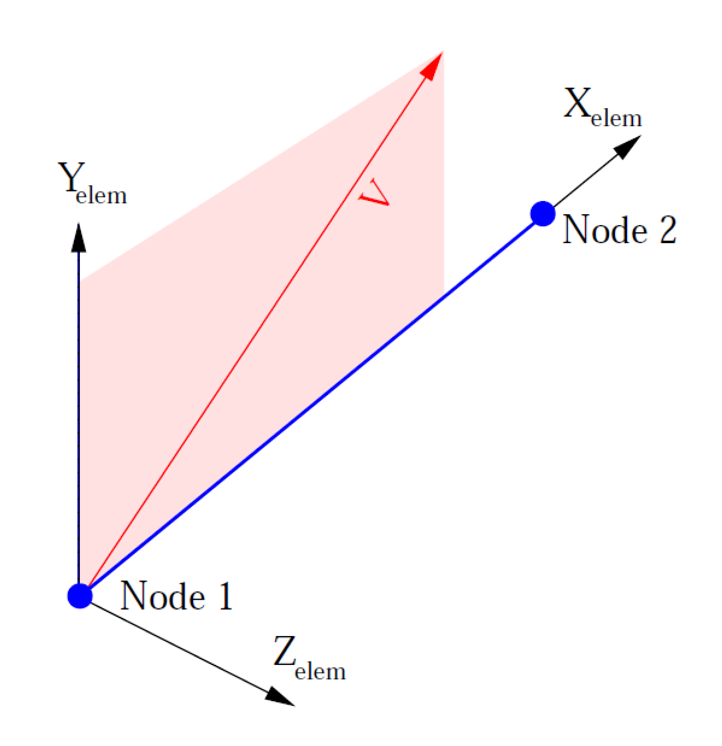
Fig. 6.23 User mounted coordinate system.

6.2.15.3. Mount Output Variables

The user mount defines a number of specific element output variables.

• user_mount_r_axis, user_mount_s_axis, user_mount_t_axis: vector quantities that can be used to visualize the user mount coordinate system ensuring it is setup and rotated as expected.

• element_state_variables: state variables used for the mount computations. The state variable array size and meaning will vary based on the user subroutine calls and/or mount type

6.2.15.4. Mount Sizing Routine

The host code must allocate memory in which to read the parameters associated with each mount and the state variables used by the mount. For a given mount type these sizes must be constant, but the size can vary on different types of mounts. The mount sizing routine is used to define these sizes and has the following definition.

SUBROUTINE SIZE_MOUNT:

  INPUT DATA:
    NONE

  OUTPUT DATA:
    INTEGER nParam: The number of parameters used to define each
                    mount. For example gap length in a gap element

    INTEGER nState: The number of state variables used by the
                    mount.

    INTEGER nActive: An indicator of which degrees of freedom are
                     active. This integer is a logical sum of
                     contributions from each dof, where X=1, Y=10,
                     Z=100, RotX=1000, RotY=10000, RotZ=100000. Thus,
                     a mount that couples only translations has
                     nActive=111, while a mount with only rotations
                     is 1. A mount with all six is 111111.

  RESTRICTIONS:
    For a given mount type the sizing routine must always return the
    same number of parameters and number of state variables. Note,
    This routine may be called by the host code at any time, for example
    at initialization or immediately before writing a restart file.

6.2.15.5. Mount Initialization Routine

The mount initialize routine provides an opportunity for the mount to set its initial state data. The host code will call the mount initialize routine once at the start of the run. The mount initialize routine will be called on each mount element individually.

SUBROUTINE INITIALIZE_MOUNT:

  INPUT DATA:
    REAL startTime: The analysis time at the start of the first analysis
                    load step or time step.

    REAL X_Elem(3): Mount inputs and outputs will be defined in a local
                    coordinate system computed by the host code. X_Elem
                    is a vector aligned with the mount element. Y_elem
                    and Z_elem are orthogonal to X_Elem. The origin of
                    the element coordinate system is located at the
                    first node of the mount element, with X_Elem as the
                    unit vector of the element coordinate system in
                    global XYZ coordinates. Based on mount
                    configuration at start of analysis.

    REAL Y_Elem(3): Unit vector of the element coordinate system in
                    global XYZ coordinates. Based on mount configuration
                    at start of analysis.

    REAL Z_Elem(3): Unit vector of the element coordinate system in
                    global XYZ coordinates. Based on mount configuration
                    at start of analysis.

    REAL coord1(6): The element coordinates of node 1 on the mount at
                    the beginning of the analysis. Order is
                    (translational_x, translational_y, translational_z,
                    rotational_x, rotational_y, rotational_z)

    REAL coord2(6): The element coordinates of node 2 on the mount at
                    the beginning of the analysis.

    REAL param(nParam): The parameters associated with the current mount
                        element. These parameters may be set in the
                        input deck or read from the mesh file
                        attributes. The number of parameters read by
                        the host code and passed to this routine is the
                        same 'nParam' value that is defined by the
                        'SIZE_MOUNT' routine.

  OUTPUT DATA:
    REAL sNew(nState): The initial mount state variables at the start of
                       the analysis. The number of state variables
                       passed out is the same 'nState' value that is
                       defined by the 'SIZE_MOUNT' routine.

    REAL Z_ElemOut(3): The X_Elem of the local coordinate system will
                      always be mount aligned. Element frame is always
                      orthogonal. The host code will compute a valid
                      element coordinate system and pass it to the
                      initialization routine. The mount initialize
                      routine may modify the initial layout of the
                      element coordinate system by passing back a new
                      Z_Elem in Z_ElemOut. Z_ElemOut is defined in
                      global XYZ coordinates. Note, the Z_Elem used by
                      the host code must be orthogonal to X_Elem. If
                      Z_ElemOut is not orthogonal to X_Elem the host
                      code will update it such that: Y_Elem =
                      Cross(Z_ElemOut, X_Elem), and Z_Elem =
                      Cross(X_Elem, Y_Elem)

    INTEGER errorCode: If the mount routine completed without hitting
                       any errors the errorCode should be set to zero. A
                       positive errorCode indicates the mount routine
                       hit a fatal error. If a mount returns a fatal
                       error the host code will report the mount ID and
                       errorCode in the log file and then abort
                       execution gracefully as soon as possible. A
                       negative errorCode indicates the mount hit a non
                       fatal warning. If a mount returns a warning code
                       the host code will report the mount ID and
                       errorCode in the log file and continue execution.

  RESTRICTIONS:
    a) The mount initialize routine may not modify in any way any of the
       input arguments. Any such changes will at best be ignored and at
       worst may corrupt the host code's database causing unpredictable
       results.

    b) The mount initialize routine must never call abort or stop, if
       the mount encounters an error it must return an error code.

    c) The mount must explicitly set all output variables. All sNew
       values should always be set to something. The mount should always
       set the errorCode to something (zero if routine executed without
       any errors). If the mount just uses the default local coordinate
       system, initialize routines should copy "Orient" into
       "OrientOut."

    d) The mount initialize routine must not make any parallel calls and
       should not be aware that it is running in parallel or running on
       a specific processor (the host code may move it from one
       processor to another during the run).

    e) Reading or writing to/from any files within the mount code is
       highly discouraged. If done the file should be opened and closed
       each call rather than left open.

    f) The mount must not store any recoverable information in any
       location other than the state variables that are passed out of he
       INITIALIZE MOUNT routine. For example the mount routine should
       not set and then retrieve a static variable or attempt to do its
       own memory allocation and data storage.

6.2.15.6. Mount Execution Routine

The host code will call the mount execute routine any time the mount force must be evaluated. The mount execute routine takes as input the state of the mount at the beginning of a load step or time step. The execute routine returns the force in the mount during the load step. The execute routine should also update any internal mount state variables to the end of load step values. The mount execute routine will be called on each mount element individually. Note the mount execute routine may be called several times during a load step, for example for use in an iterative solver.

SUBROUTINE COMPUTE_MOUNT_FORCE:

  INPUT DATA:
    REAL startTime: The analysis time at the start of the current
                    analysis load step or time step.

    REAL deltaT: The length of the current analysis time step or load
                 step. Note, the code may call the mount execute routine
                 to probe the mount stiffness, if that is the
                 case the deltaT passed in for the probe may be 0.0.

    REAL X_Elem(3): Mount inputs and outputs will be defined in a local
                    element coordinate system. X is a vector aligned
                    with the mount element. Y and Z are orthogonal to
                    X. The origin of the element coordinate system is
                    located at the first node of the mount element. The
                    host code will update the element coordinate system
                    if the mount element undergoes rotation. Vectors
                    defined in the mount configuration at end of load
                    step.

    REAL Y_Elem(3): Unit Y vector of the element coordinate system in
                    global XYZ coordinates. Based on mount configuration
                    at end of load step.


    REAL Z_Elem(3): Unit Z vector of the local coordinate system in
                    global XYZ coordinates. Based on mount configuration
                    at end of load step.

    REAL coord1(6): The element coordinates of node 1 on the mount at
                    the end of the load step. Order is (translational_x,
                    translational_y, translational_z, rotational_x,
                    rotational_y, rotational_z)

    REAL coord2(6): The element coordinates of node 2 on the mount at
                    the end of the load step.

    REAL disp1(6): The element displacement of node 1 at the end of the
                   load step.

    REAL disp2(6): The element displacement of node 2 at the end of the
                   load step.

    REAL vel1(6): The element velocity of node 1 at the middle of the
                  load step.

    REAL vel2(6): The element velocity of node 2 at the middle of the
                  load step.

    REAL param(nParam): The parameters associated with the current mount
                        element. These parameters may be set in the
                        input deck or read from the mesh file
                        attributes. The number of parameters read by
                        the host code and passed to this routine is the
                        same 'nParam' value that is defined by the
                        'SIZE_MOUNT' routine.

    REAL sOld(nState): The mount state variables at the start of the
                       load step. The number of state variables passed
                       in is the same 'nState' value that is defined by
                       the 'SIZE_MOUNT' routine.

  OUTPUT DATA:

    REAL force1(6): The element coordinate forces and moments at node 1
                    at the end of the load step.

    REAL force2(6): The element coordinate forces and moments at node 2
                    during the load step.

    REAL sNew(nState): The updated mount state variables at the end of
                       the load step. The number of state variables
                       passed out is the same 'nState' value that is
                       defined by the 'SIZE_MOUNT' routine.

    INTEGER errorCode: If the mount routine completed without hitting
                       any errors the errorCode should be set to zero. A
                       positive errorCode indicates the mount routine
                       hit a fatal error. If a mount returns a fatal
                       error the host code will report the mount ID and
                       errorCode to the user then abort execution
                       gracefully as soon as possible. A negative
                       errorCode indicates the mount hit a non fatal
                       warning. If a mount returns a warning code the
                       host code will report the mount ID and errorCode
                       to the user and continue execution.

  RESTRICTIONS:
    a) The mount execute routine may not modify in any way any of the
       input arguments. Any such changes will at best be ignored and at
       worst may corrupt the host code's database causing unpredictable
       results.

    b) The mount execute routine must never call abort or stop, if the
       mount encounters an error it must return an error code.

    c) The mount must explicitly set all output variables. The return
       force should be set to zero if there is no force. sOld values
       should be copied into sNew if the mount state variables were not
       changed. The mount should always set the errorCode to something
       (zero if routine executed without any errors).

    d) The mount execute routine must not make any parallel calls and
       should not be aware that it is running in parallel or running on
       a specific processor (the host code may move it from one
       processor to another during the run).

    e) Reading or writing to/from any files within the mount code is
       highly discouraged.

    f) The mount must not store any recoverable information in any
       location other than the state variables that are passed into and
       out of the COMPUTE MOUNT FORCE routine. For example the mount
       routine should not set and then retrieve a static variable or
       attempt to do its own memory allocation and data storage.

6.2.15.7. Example

The following is an example of use of the API for defining a simple mount. This example is written in Fortran 77. The mount designed here is a truss element with a failure criterion. The truss element behaves as a linear spring. If the strain in the truss becomes too large the truss breaks. A broken truss can never again support tensile or compressive loads even if later the strain is reduced below the break strain value.

//=================================================================
      subroutine fail_truss_size(int nParam, int nState, int nActive)
      int nParam
      int nState
c
c Param(1) is the stiffness of the truss, expressed in force per strain
c Param(2) is the critical value of tensile strain at which the truss
c breaks.
c
      nParam = 2
c
c State(1) is the initial length of the truss State(2) indicates if the
c truss is broken or not, 1 is intact, 2 is broken
c
      nState = 2
c Truss does not couple to rotation,
      nActive = 111
      end
//=================================================================
subroutine fail_truss_initialize(startTime,
     &                           X_Elem, Y_Elem, Z_Elem,
     &                           coord1, coord2, param,
     &                           sNew, Z_ElemOut, errorCode)
c
c Input arguments
c
      double startTime
      double X_Elem(3), Y_Elem(3), Z_Elem(3)
      double coord1(6), coord2(6)
      double param(2)
c
c Output arguments
c
      double sNew(2)
      double Z_ElemOut(3)
      int errorCode
c
c Compute and store initial truss length, this is just the length in R
c Set the truss as initially unbroken
c
      sNew(1) = fabs(coord1(1)-coord2(1))
      sNew(2) = 1
c
c If truss is initially zero length, problem ill defined, abort
c
      if(sNew(1) == 0.0) then
        errorCode = 1
        return
      endif
c
c Use default element coordinate system
c
      Z_ElemOut(1) = Z_Elem(1)
      Z_ElemOut(2) = Z_Elem(2)
      Z_ElemOut(3) = Z_Elem(3)
      errorCode = 0
      end
//=================================================================
subroutine fail_truss_compute(startTime, deltaT,
     &                        X_Elem, Y_Elem, Z_Elem,
     &                        coord1, coord2,
     &                        disp1, disp2,
     &                        vel1, vel2,
     &                        param,
     &                        sOld,
     &                        force1, force2,
     &                        sNew,
     &                        errorCode)
c
c Input arguments
c
      double startTime, deltaT
      double X_Elem(3), Y_Elem(3), Z_Elem(3)
      double coord1(6), coord2(6)
      double disp1(6), disp2(6)
      double vel1(6), vel2(6)
      double param(2)
      double sOld(2)
c
c Output arguments
c
      double force1(6), force2(6)
      double sNew(2)
      int errorCode
c
c Local variables
c
      double newLen
      double curStrain
      double curForce
c
c Check if truss is 'broken' if so it no force
c
      if(sOld(2) == 2) then
        force1(1) = 0.0
        force1(2) = 0.0
        force1(3) = 0.0
        force1(4) = 0.0
        force1(5) = 0.0
        force1(6) = 0.0
        force2(1) = 0.0
        force2(2) = 0.0
        force2(3) = 0.0
        force2(4) = 0.0
        force2(5) = 0.0
        force2(6) = 0.0
        sNew(1) = sOld(1)
        sNew(2) = sOld(2)
        errorCode = 0
        return
      endif
c
c Compute the new truss length, this is just the length in R
c
      newLen = fabs(coord1(1)- coord2(1))
c
c If length compressed to zero, element is invalid, make host code abort
c
      if(newLen == 0.0) then
        errorCode = 1
        return
      endif
c
c Compute the current strain as new length over original length.
c Compute tensile (positive) or compressive (negative) force based on
c stiffness time strain. Force is applied along R with now off axis
c component. If strain exceeds critical value break the truss
c
      curStrain = (newLen/sOld(1))
      if(curStrain > param(2)) then
        sNew(2) = 2
        force1(1) = 0.0
        force1(2) = 0.0
        force1(3) = 0.0
        force1(4) = 0.0
        force1(5) = 0.0
        force1(6) = 0.0
        force2(1) = 0.0
        force2(2) = 0.0
        force2(3) = 0.0
        force2(4) = 0.0
        force2(5) = 0.0
        force2(6) = 0.0
        sNew(1) = sOld(1)
      else
        if(curStrain > 1.0) then
          curForce = (curStrain-1.0) * param(1)
        else
          curForce = -(1.0/curStrain) * param(1)
        endif
        force1(1) = curForce
        force1(2) = 0.0
        force1(3) = 0.0
        force1(4) = 0.0
        force1(5) = 0.0
        force1(6) = 0.0
        force2(1) = -curForce
        force2(2) = 0.0
        force2(3) = 0.0
        force2(4) = 0.0
        force2(5) = 0.0
        force2(6) = 0.0
        sNew(1) = sOld(1)
        sNew(2) = sOld(2)
      endif
      errorCode = 0
      end

6.2.16. Cylindrical Joint

BEGIN CYLINDRICAL JOINT SECTION <string>cylj_section_name
  AXIAL DIRECTION = <vector_3D> axial_direction
   axial direction = 0.0 0.0 -1.0
  AXIAL ROTATION STIFFNESS = <string>theta_stiffness
  AXIAL TRANSLATION STIFFNESS = <string>axial_stiffness
  INNER SURFACE = <string>inner_surface
  OUTER SURFACE = <string>outer_surface
  RADIAL ROTATION STIFFNESS = <string>yaw_stiffness
  RADIAL TRANSLATION STIFFNESS = <string>radial_stiffness
END [CYLINDRICAL JOINT SECTION <string> truss_section_name]

The CYLINDRICAL JOINT SECTION command block provides the ability to add nonlinear stiffness against the relative average motion of two surfaces (inner_surface and outer_surface) using a cylindrical system assumption. (In contrast, to kinematically prescribe a cylindrical boundary condition a user should use the CYLINDRICAL AXIS line command within a prescribed kinematic boundary condition command block, e.g., for prescribed displacement see Section 7.4.2.2.) The cylindrical joint capability is intended for modeling joints with cylindrical constraints (e.g., a disc mounted on a post) and it works best on joints that are axisymmetric or nearly so. In addition, unspecified stiffness are assumed to be zero for these joints so that free motion may be specified (e.g., a disc free to rotate on a post which has zero AXIAL ROTATION STIFFNESS, while all other stiffness are specified).

This command block should be referenced in an element block of a single three-dimensional two node element (i.e., a bar or beam element in typical meshing tools). The two node element is used to define the reference axis against which the relative motion of the two surfaces is computed. The element variables for this section type are listed in Table 6.4 and are stored on the single two node element.

The element variables cylj_rst_origin, cylj_r_axis, cylj_s_axis, and cylj_t_axis can be used to visualize the local co-rotational Cartesian reference axes, which is constructed in much the same way as for beam or bar elements. The value of cylj_rst_origin is at the center of the two node element and the cylj_r_axis is in the direction from first node to the second node as defined by the two node element connectivity (note that the cylj_r_axis is not the radial direction). The directions cylj_s_axis and cylj_t_axis are internally computed and are orthogonal to each other and cylj_r_axis.

The parameter, cylj_section_name is user-defined and is referenced by a SECTION command line in a PARAMETERS FOR BLOCK command block.

The parameter, axial_direction can optionally be input to define the direction along the axis of the cylindrical joint. Sierra/SM will take this direction and determine if the normal of the beam element needs to be swapped to the opposite direction. If the command is not present, the beam normal will be used.

The function defined with theta_stiffness on the command line AXIAL ROTATION STIFFNESS is used to determine moment applied as a function of the two surfaces’ relative motion illustrated in Fig. 6.24.

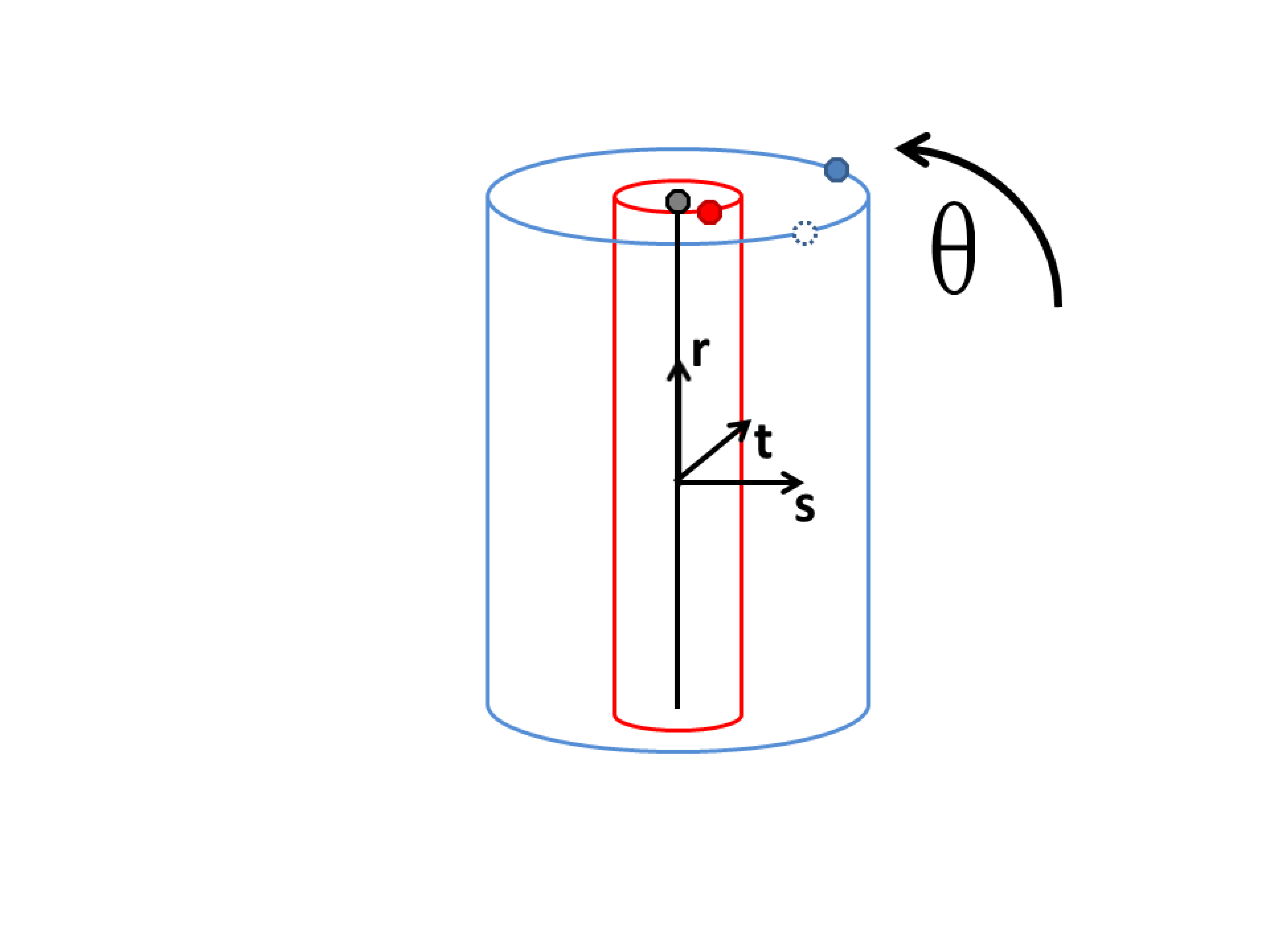
Fig. 6.24 Cylindrical joint axial rotation.

The function defined with axial_stiffness on the command line AXIAL TRANSLATION STIFFNESS is used to determine force applied as a function of the two surfaces’ relative motion illustrated in Fig. 6.25.

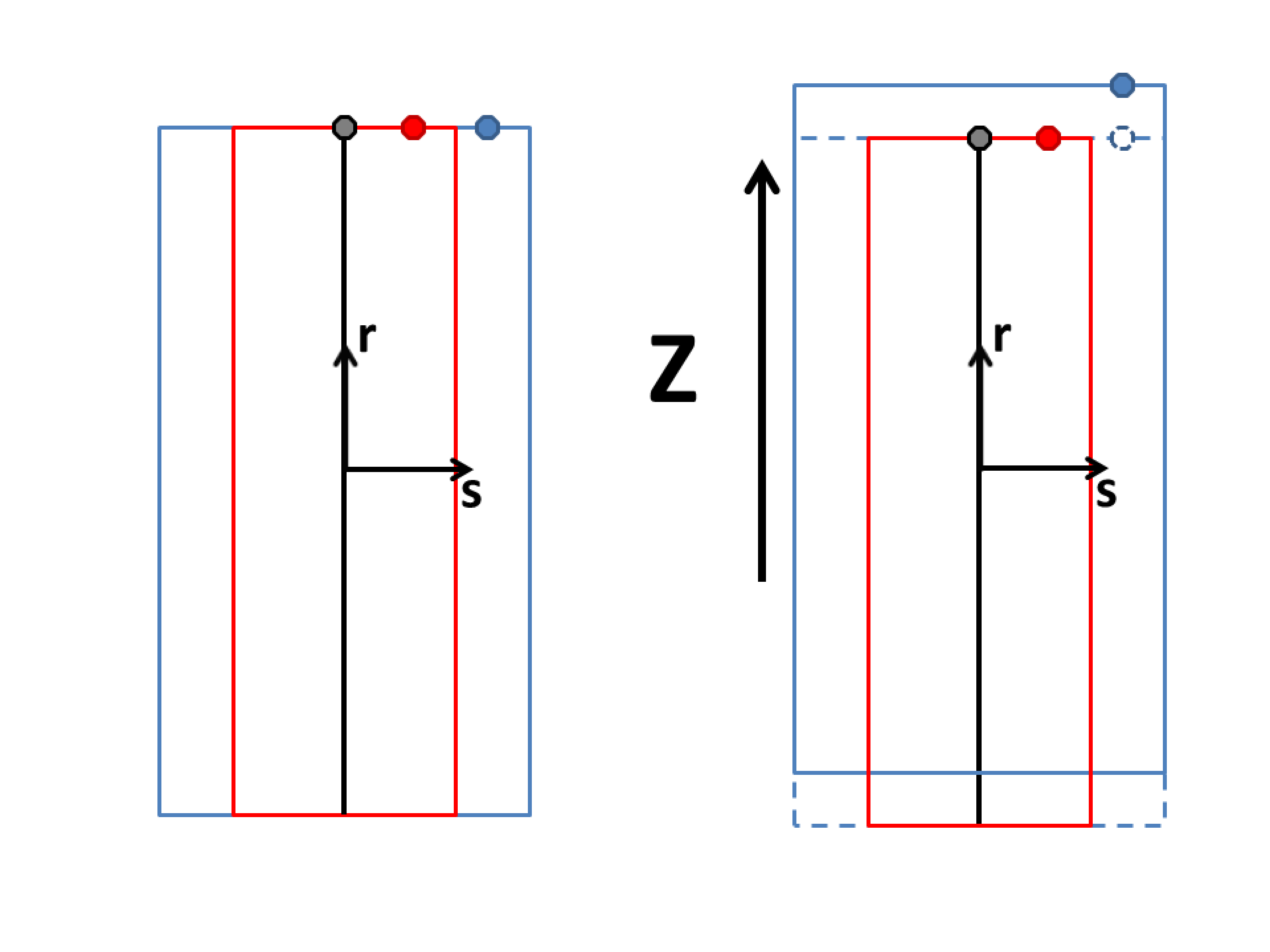
Fig. 6.25 Cylindrical joint axial translation.

The function defined with yaw_stiffness on the command line RADIAL ROTATIONAL STIFFNESS is used to determine moment applied as a function of the two surfaces’ relative motion illustrated in Fig. 6.26. This function should generally start at (0,0) and increase monotonically positive X positive Y quadrant.

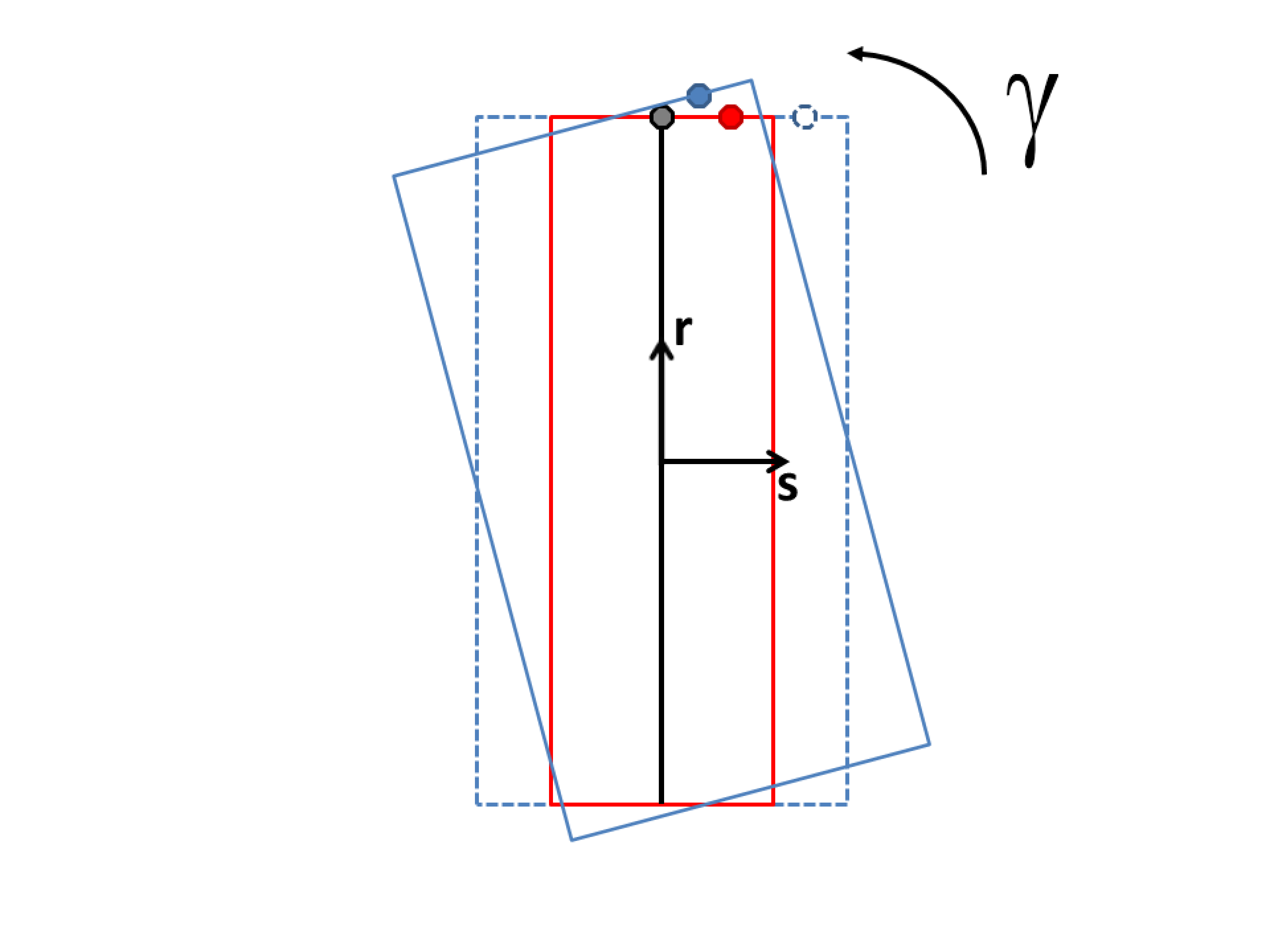
Fig. 6.26 Cylindrical joint radial rotation.

The function defined with radial_stiffness on the command line RADIAL TRANSLATION STIFFNESS is used to determine force applied as a function of the relative motion illustrated in Fig. 6.27. This function should generally start at (0,0) and increase monotonically positive X positive Y quadrant.

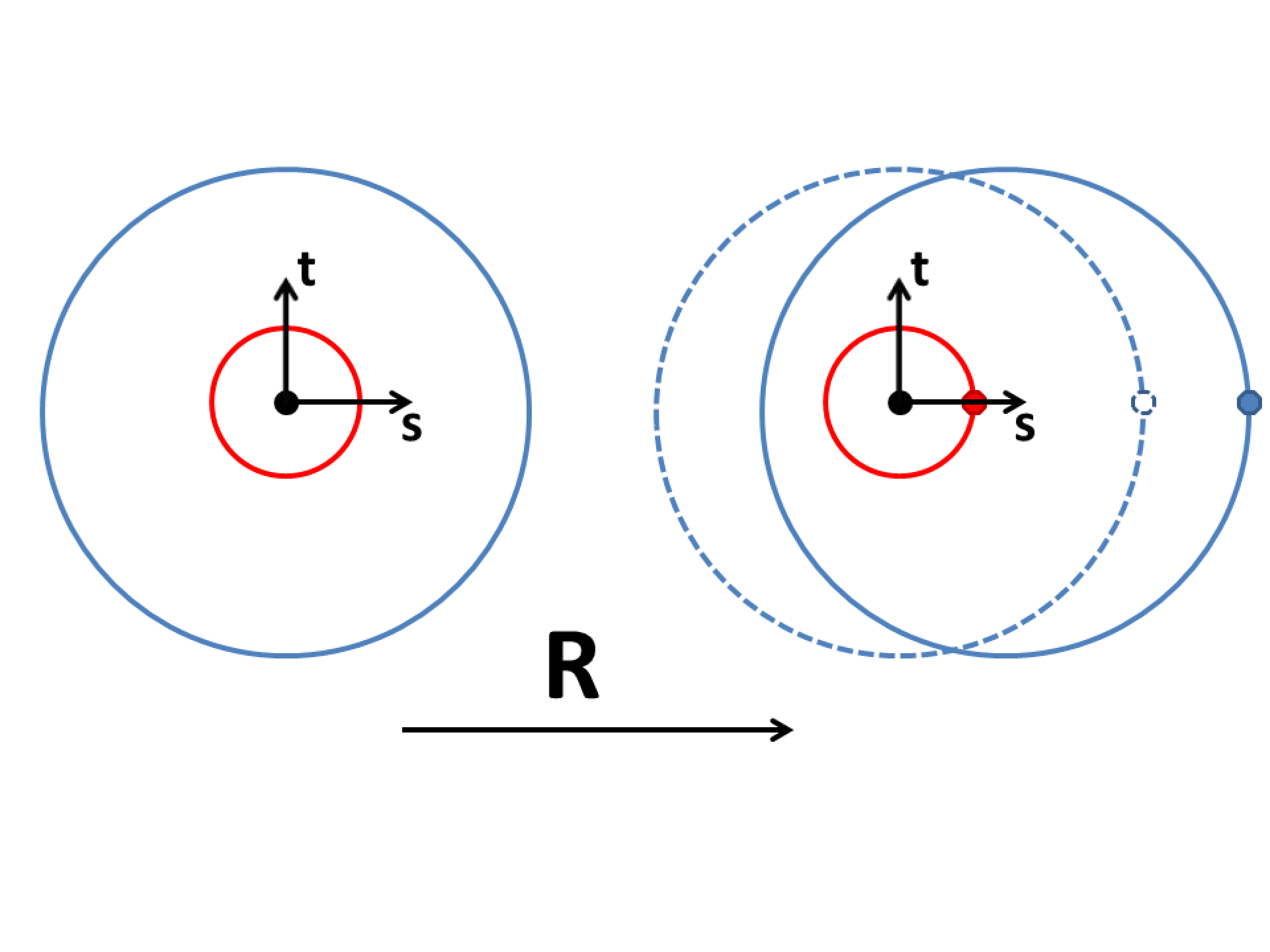
Fig. 6.27 Cylindrical joint radial translation.

The INNER SURFACE and OUTER SURFACE commands specify the surfaces where relative motion is measured and the resulting force and moments are distributed. In a given time step, the averaged step motion in the reference Cartesian coordinate system is computed on the inner_surface and outer_surface. The accumulated translational and rotational motion is stored in the three-component vector element variables cylj_rst_coord1 and cylj_rst_theta1, respectively, for the inner_surface. Similarly, the accumulated motion for outer_surface is stored in cylj_rst_coord2 and cylj_rst_theta2.

The relative motion used for evaluating the stiffness functions is calculated by the vector math of (cylj_rst_coord2 - cylj_rst_coord1) and (cylj_rst_theta2 - cylj_rst_theta1). The relative motion of the coord values is used with the translational stiffness and the resulting force is stored in the element variable cylj_rst_force. Similarly, the theta values use the rotational stiffness and result in a moment stored in cylj_rst_moment. The element internal force and moment values are then applied equally and of opposite sign to the inner_surface and outer_surface and are distributed across each surface’s nodes for the cylindrical joint element’s internal force.

For output the “x” vector components of the coord, theta, force, and moment element variables correspond to the axial direction cylj_r_axis ``. The "y" and "z" components correspond to the ``cylj_s_axis and cylj_t_axis radial directions respectively, which are treated with the same translational and rotational stiffness due to the axisymmetric assumption.

Table 6.4 Variables For Cylindrical Joint

Variable Name	Type	Comments
cylj_rst_origin	Vector_3D	( Reference axis origin )
cylj_r_axis	Vector_3D	( Reference axis r direction )
cylj_s_axis	Vector_3D	( Reference axis s direction )
cylj_t_axis	Vector_3D	( Reference axis t direction )
cylj_rst_coord1	Vector_3D	( Inner surface translational coordinates )
cylj_rst_theta1	Vector_3D	( Inner surface rotational coordinates )
cylj_rst_coord2	Vector_3D	( Outer surface translational coordinates )
cylj_rst_theta2	Vector_3D	( Outer surface rotational coordinates )
cylj_rst_force	Vector_3D	( Translational force vector )
cylj_rst_moment	Vector_3D	( Rotational moment vector )

Warning

The cylindrical joint element has no mass and only increases the stiffness of the nodes in inner_surface and outer_surface. This additional stiffness is currently not reflected in the computation of the stable time step. A time step scale factor may be required to obtain a stable time step if nodes in the cylindrical joint are part of the element that is controlling the time step. No checks are made of the validity of the stiffness functions provided but the functions should only have values in the upper right and lower left quadrants of a force versus displacement or moment versus rotation plot.

---

[1] (1,2)

M.M. Rashid. Incremental kinematics for finite element applications. International Journal for Numerical Methods in Engineering, 36:3937–3956, 1993. doi:10.1002/nme.1620362302.

[2] (1,2,3)

T.A. Laursen, S.W. Attaway, and R.I. Zadoks. SEACAS theory manuals: part III. finite element analysis in nonlinear solid mechanics. Technical Report SAND98-1760/3, Sandia National Laboratories, Albuquerque, NM, 1999. URL: http://infoserve.sandia.gov/sand_doc/1998/981760-3.pdf.

[3]

C.R. Dohrman, M.W. Heinstein, J. Jung, S.W. Key, and W.R. Witkowski. Node-based uniform strain elements for three-node triangular and four-node tetrahedral meshes. International Journal for Numerical Methods in Engineering, 47:1549–1568, 2000. doi:10.1002/(SICI)1097-0207(20000330)47:9<1549::AID-NME842>3.0.CO;2-K.

[4]

K.-J. Bathe. Finite element formulations for large deformation dynamic analysis. International Journal for Numerical Methods in Engineering, 9:353–386, 1975.

[5]

J.T. Ostien, J.W. Foulk, A. Mota, and M.G. Veilleux. A 10-node composite tetrahedral finite element for solid mechanics. International Journal for Numerical Methods in Engineering, 2016.

[6]

R. L. Taylor and E. Artioli. VEM for Inelastic Solids, pages 381–394. Springer International Publishing, Cham, 2018. doi:10.1007/978-3-319-60885-3_18.

[7] (1,2,3)

Q. Yang, A. Mota, and M. Ortiz. A class of variational strain-localization finite elements. International Journal for Numerical Methods in Engineering, 62:1013–1037, 2005. doi:10.1002/nme.1199.

[8]

T. Belytschko and I. Leviathan. Physical stabilization of the 4-node shell element with one point quadrature. Computer Methods in Applied Mechanics and Engineering, 113:321–350, 1994.

[9]

T. Belytschko and I. Leviathan. Projection schemes for one-point quadrature shell elements. Computer Methods in Applied Mechanics and Engineering, 115:277–286, 1994.

[10]

P. Madabhusi-Raman and J.F. Davalos. Static shear correction factor for laminated rectangular beams. Composites Part B: Engineering, 27(3):285–293, 1996. doi:10.1016/1359-8368(95)00014-3.

[11]

G.D. Sjaardema. Overview of the Sandia National Laboratories engineering analysis code access system. Technical Report SAND92-2292, Sandia National Laboratories, Albuquerque, NM, January 1993. URL: http://infoserve.sandia.gov/sand_doc/1992/922292.pdf.

[12]

J.W. Swegle, S.W. Attaway, M.W. Heinstein, F.J. Mello, and D.L. Hicks. An analysis of smoothed particle hydrodynamics. Technical Report SAND93-2513, Sandia National Laboratories, Albuquerque, NM, March 1994. URL: http://infoserve.sandia.gov/sand_doc/1993/932513.pdf.

[13]

L.M. Taylor and D.P. Flanagan. Pronto3D: a three-dimensional transient solid dynamics program. Technical Report SAND87-1912, Sandia National Laboratories, Albuquerque, NM, March 1989. URL: http://infoserve.sandia.gov/sand_doc/1987/871912.pdf.

[14]

J. Monaghan. SPH without a tensile instability. Journal of Computational Physics, 159(2):290–311, 2000. doi:10.1006/jcph.2000.6439.