6.1. Finite Element Model

BEGIN FINITE ELEMENT MODEL <string>mesh_descriptor
  DATABASE NAME = <string>mesh_file_name
  DATABASE TYPE = <string>database_type(exodusII)
  ALIAS <string>mesh_identifier AS <string>user_name
  OMIT BLOCK <string>block_list
  OMIT ASSEMBLY <string>assembly_list
  COMPONENT SEPARATOR CHARACTER = <string>separator
  TIME SCALE FACTOR = <real>timeScaleFactor
  DECOMPOSITION METHOD = RCB|RIB|LINEAR|HSFC|BLOCK|CYCLIC|
    RANDOM|KWAY|GEOM_KWAY|KWAY_GEOM|METIS_SFC|EXTERNAL

  BEGIN BLOCK DEFAULTS
    #
    #  Set default values for each 'PARAMETERS FOR
    #  BLOCK' command
    #
  END [BLOCK DEFAULTS]

  BEGIN PARAMETERS FOR BLOCK [<string list>block_names|assembly_names]
    #
    # Command lines that define attributes for
    # a particular element block appear in this
    # command block.
    #
  END [PARAMETERS FOR BLOCK <string list>block_names|assembly_names]

  BEGIN ASSEMBLY <string>assembly_name
    #
    # Command lines that list the mesh objects
    # that are to be included in the assembly of blocks,
    # 'assembly_name'.
    #
  END ASSEMBLY [<string>assembly_name]
END [FINITE ELEMENT MODEL <string>mesh_descriptor]

The input file must point to a mesh file that is to be used for an analysis. The name of the mesh file appears within a FINITE ELEMENT MODEL command block, which appears in the SIERRA scope. In this command block, the particular mesh file that describes the model is identified. There will also be one or more PARAMETERS FOR BLOCK command blocks in this block. (All the PARAMETERS FOR BLOCK command blocks are embedded in the FINITE ELEMENT MODEL command block.) A material type and model, a section, and various other parameters for the element block or assembly of element blocks are set within the PARAMETERS FOR BLOCK command block. The concept of “section” is explained in Section 6.1.7. Assemblies are created in the BEGIN ASSEMBLY command block.

The following element types are supported in Sierra/SM{} analyses:

• Eight-node, uniform-gradient hexahedron Both a midpoint-increment formulation [[1]] and a strongly objective formulation are implemented [[2]]. These elements can be used with any of the material models described in Section 5.

• Six-node, uniform-gradient wedge Both a midpoint-increment formulation [[1]] and a strongly objective formulation are implemented [[2]]. These elements can be used with any of the material models described in Section 5.

• Five-node, uniform-gradient pyramid Both a midpoint-increment formulation [[1]] and a strongly objective formulation [[2]] are implemented. These elements can be used with any of the material models described in Section 5.

• Eight-node, selective-deviatoric hexahedron The strongly objective formulation is recommended. Midpoint increment strain incrementation is available for legacy compatibility. This element can be used with any of the material models described in Section 5. The selective-deviatoric integration rule is specified in the BEGIN SOLID SECTION command block using the FORMULATION command line as described in Table 6.3.

• Eight, twenty, and twenty seven noded, total-Lagrangian hexahedra The total-Lagrangian hexahedra are fully integrated elements with optional \(J\)-averaging to control pressure modes in incompressible media. These elements can be used with any of the material models described in Section 5. They are described in Section 6.2.2.

• Four-node tetrahedron There is now the regular element formulation for the four-node tetrahedron and a node-based formulation for the four-node tetrahedron. For the regular element formulation, only a strongly objective formulation is implemented. The concept of a node-based four-node tetrahedron is described in [[3]]. The regular four-node tetrahedron can be used with any of the material models described in Section 5. The node-based tetrahedron can be used with any of the material models described in Section 5. When using node-based tetrahedron it is important that nodal quantities are used where other element types use element quantities. For example, element variable stress is evaluated with a regular four-node tetrahedron, but in node-based tetrahedron one should use nodal variable element_stress_##, where ## is a one-based integer \(>0\). Nodal variables for node-based tetrahedra will exist on all nodes but are zero where they are not used. Element variables for node-based elements serve as intermediate variables and should not be used in post-processing in the same way as other regular element variables.

• Four and ten-noded, total-Lagrangian tetrahedra The total-Lagrangian tetrahedra are fully integrated elements with optional \(J\)-averaging to control pressure modes in incompressible media. These elements can be used with any of the material models described in Section 5. They are described in more detail in Section 6.2.2.

• Ten-node, composite tetrahedron The composite tet is now the default ten-node tet element in Sierra/SM. This element can be used with any of the material models described in Section 5. This element can be used by creating an empty solid section, by not specifying a section in the block definition, or by using a Total Lagrange section. See Section 6.2.2 for more details.

• Thirteen-node, total-Lagrangian pyramid The total-Lagrangian pyramid is a fully integrated element with optional \(J\)-averaging to control pressure modes in incompressible media. These elements can be used with any of the material models described in Section 5. They are described in more detail in Section 6.2.2.

• Fifteen node, total-Lagrangian wedge The total-Lagrangian wedge is a fully integrated element with optional \(J\)-averaging to control pressure modes in incompressible media. These elements can be used with any of the material models described in Section 5. They are described in more detail in Section 6.2.2.

• Ten-node, fully-integrated tetrahedron Only a strongly objective formulation is implemented. This element can be used with any of the material models described in Section 5. The full integration rule is specified in the BEGIN SOLID SECTION command block using the FORMULATION command line as described in Table 6.3.

• Four-node, quadrilateral, uniform-gradient membrane Both a midpoint-increment formulation and a strongly objective formulation are implemented. This element is derived from the Key-Hoff shell formulation [[4]]. The strongly objective formulation has not been extensively tested, and it is recommended that the midpoint-increment formulation, which is the default, be used for this element type. These elements can be used with any of the following material models described in Section 5:

  • Elastic

  • Elastic-plastic

  • Elastic-plastic power-law hardening

  • Multilinear elastic-plastic hardening (no failure)

• Four-node, quadrilateral shell This shell uses the Key-Hoff formulation [[4]]. Both a midpoint-increment formulation and a strongly objective formulation are implemented. The strongly objective formulation has not been extensively tested, and it is recommended that the midpoint-increment formulation, which is the default, be used for this element type. These elements can be used with any of the following material models described in Section 5:

  • Elastic

  • Elastic-plastic

  • Elastic-plastic power-law hardening

  • Multilinear elastic-plastic hardening without failure

  • Multilinear elastic-plastic hardening with failure

• Four-node, quadrilateral, selective-deviatoric membrane Only a midpoint-increment formulation is implemented. These elements can be used with any of the following material models described in Section 5:

  • Elastic

  • Elastic-plastic

  • Elastic-plastic power-law hardening

  • Multilinear elastic-plastic hardening (no failure)

• Linear elastic shell The linear elastic shell element is linear in both a material and geometric sense. The linear elastic shell element can be used with any material, however it will use only the density and elastic material constants of that material. Use of the linear elastic shell element is specified with the FORMULATION = NQUAD command in the section command block.

• Three-node, triangular shell This shell uses the same formulation as the three-node triangular shell in Pronto [[1]]. A midpoint-increment formulation is implemented. This element can be used with any of the following material models described in Section 5:

  • Elastic

  • Elastic-plastic

  • Elastic-plastic power-law hardening

  • Multilinear elastic-plastic hardening without failure

  • Multilinear elastic-plastic hardening with failure

• Two-node beam The beam element is a uniform result model. Strains and stresses are computed only at the midpoint of the element. These midpoint values determine the forces and moments for the beam. The beam element is based on an incremental kinematic formulation that is accurate for large strains and rotations (i.e., this element exactly agrees with a logarithmic strain formulation under large strain axial loading). Thinning of the cross section is taken into account through a constant volume assumption. There are several different sections currently implemented for the beam including rod, tube, bar, box, and I.’ This element can be used with any of the following material models described in :numref:`materials:

  • Elastic

  • Elastic-plastic

• Two-node truss The two-node truss element carries only a uniform axial stress. Currently, there is a linear-elastic material model for the truss element.

• Two-node spring The two-node spring element computes a uniaxial resistance force based on a nonlinear force-engineering strain function. This element can handle preloads, mass per unit length, resetting of the initial length after preload and any arbitrary loading function.

• Two-node damper The two-node damping element computes a damping force based on the relative velocity of the two nodes along the axis of the element. This element uses only a damping parameter for a material property.

• Point mass The point mass element allows the user to put a specified mass and/or rotational inertia at a single node. This element requires input for density, but does not make use of any other material properties.

• Particle The particle element is a zero-dimensional, sphere-topology element which may be used with any of the material models described in Section 5.

The command block to describe a mesh file begins with

BEGIN FINITE ELEMENT MODEL <string>mesh_descriptor

and is terminated with

END [FINITE ELEMENT MODEL <string>mesh_descriptor]

where mesh_descriptor is a user-selected name for the mesh. This section discusses the command lines within the scope of the FINITE ELEMENT MODEL command block but outside the scope of the PARAMETERS FOR BLOCK command block, as well as the PARAMETERS FOR BLOCK command block and the associated command lines for this particular block.

6.1.1. Identification of Mesh File

Nested within the FINITE ELEMENT MODEL command block are two command lines (DATABASE NAME and DATABASE TYPE) that give the mesh name and define the type for the mesh file, respectively. The command line

DATABASE NAME = <string>mesh_file_name

gives the name of the mesh file with the string mesh_file_name. If the current mesh file is in the default directory and is named job.g, then this command line would appear as:

DATABASE NAME = job.g

If the mesh file is in some other directory, the command line would have to show the path to that directory. For parallel runs, the string mesh_file_name is the base name for the spread of parallel mesh files. For example, for a four-processor run, the actual mesh files associated with a base name of job.g would be job.g.4.0, job.g.4.1, job.g.4.2, and job.g.4.3. The database name on the command line would be job.g.

Two meta-characters can appear in the name of the mesh file. If the %P character is found in the name, it will be replaced with the number processors being used for the run. For example, a job running on 1024 processors has the name mesh-%P/job.g, then the name would be expanded to mesh-1024/job.g and the associated mesh files would be mesh-1024/job.g.1024.0000 to mesh-1024/job.g.1024.1023. The other recognized meta-character is %B which is replaced with the base name of the input file containing the input commands. For example, if the commands are in the file my_analysis_run.i and the mesh database name is specified as %B.g, then the mesh would be read from the file my_analysis_run.g.

If the mesh file does not use the Exodus II format, the mesh file format must be specified using the command line

DATABASE TYPE = <string>database_type(exodusII)

Currently, only the Exodus II database format is supported by Presto and Adagio for mesh input. Other options may be added in the future.

6.1.2. Alias

It is possible to associate a user-defined name with some mesh entity. The mesh entity names for Exodus II entities are typically the concatenation of the entity type (for example, “block”, “nodelist”, or “surface”), an underscore (“_”), and the entity id. This generated name can be aliased to a more descriptive name by using the ALIAS command line:

ALIAS <string>mesh_identifier AS <string>user_name

This alias can then be used in other locations in the input file in place of the Exodus II name. Examples of this association are as follows:

Alias block_1   as Case
Alias block_10  as Fin
Alias block_12  as Nose
Alias surface_1 as Nose_Case_Interface
Alias surface_2 as OuterBoundary

The above examples use the Exodus II naming convention described in Section 1.6. Note that the alias may not be recognized by all code capabilities, such as contact block skinning.

6.1.3. Omit Block

If the finite element mesh contains element blocks that should be omitted from the finite element analysis, the OMIT BLOCK line command is used:

OMIT BLOCK <string>block_list

The element blocks listed in the command are removed from the model. Any node sets or surfaces only existing on nodes or elements in the omitted element blocks are also omitted. When using this command, it is necessary to deactivate (comment out) or remove any references to the omitted blocks in the rest of the input file. Note that if this command is used in a parallel analysis, it is possible for the resulting model to become unbalanced if, for example, the omitted element blocks make up a large portion of the elements on one or more processors. In this case with explicit calculations, the mesh can be rebalanced using the REBALANCE command described in Section 6.8.1.

If the block is given an alias, then that alias name must be provided to the block omission command; otherwise, the standard entity name, “block” followed by the entity id, must be used. See Section 1.6 for further discussion of the Exodus II block naming convention.

Examples of omitting element blocks are:

Omit Block block_1 block_2
Omit Block block_10
Omit Block Fin Nose

Similarly, blocks from assemblies may be omitted via the OMIT ASSEMBLY command, which will omit the blocks that comprise the assembly. The assembly must be defined only in terms of blocks; heterogeneous assemblies with entity types other than blocks are disallowed.

Warning

Both OMIT BLOCK and OMIT ASSEMBLY will ignore block and assembly names that are not found in the model.

6.1.4. Time Scale Factor

The TIME SCALE FACTOR command is used to put a uniform scale factor on the time stamps in the input mesh database. This command will have an effect on capabilities such as READ VARIABLE (Section 7.3.5) that reads boundary condition data from the input mesh.

6.1.5. Component Separator Character

A variable defined on the mesh database can be used as an initial condition, or a prescribed temperature with the READ VARIABLE command. If the variable is a vector or a tensor, then the base name of the variable will be separated from the suffixes with a separator character. The default separator character is an underscore, but it can be changed with the COMPONENT SEPARATOR CHARACTER command.

COMPONENT SEPARATOR CHARACTER = <string>character|NONE

For example, the variable displacement can have the suffixes x, y, etc. By default, the base name is separated from the suffixes with an underscore character, yielding displacement_x, displacement_y, etc., in the mesh file. The underscore can be replaced as the default separator by using the above command line. If the data used the period as the separator, then the command would be

COMPONENT SEPARATOR CHARACTER = .

In the displacement example the components would then appear in the mesh file as displacement.x, displacement.y, etc. The separator can be eliminated with an empty string or NONE.

6.1.6. Decomposition Method

The DECOMPOSITION METHOD command is an optional command used to specify how the mesh will be decomposed across multiple processors. This command is used in lieu of SEACAS tools such as decomp and the sierra --pre option. For more information about the different decomposition types please consult the table “Valid values for Decomposition Method” in the IOSS Documentation on the SEACAS Documentation website.

6.1.7. Element Block Parameters

BEGIN PARAMETERS FOR BLOCK [<string list>block_names|assembly_names]
  MATERIAL = <string>material_name
  MODEL = <string>model_name
  DENSITY SCALE FACTOR = <real>density_scale_factor(1.0)
  INCLUDE ALL BLOCKS
  REMOVE BLOCK = <string list>block_names
  REMOVE ASSEMBLY = <string list>assembly_names
  SECTION = <string>section_id
  LINEAR BULK VISCOSITY =
    <real>linear_bulk_viscosity_value(0.06)
  QUADRATIC BULK VISCOSITY =
    <real>quad_bulk_viscosity_value(1.20)
  HOURGLASS STIFFNESS =
    <real>hourglass_stiff_value(0.05)
  HOURGLASS VISCOSITY =
    <real>hourglass_visc_value(solid = 0.0,
      shell/membrane = 0.0)
  MEMBRANE HOURGLASS STIFFNESS =
    <real>memb_hourglass_stiff_value(0.05)
  MEMBRANE HOURGLASS VISCOSITY =
    <real>memb_hourglass_visc_value(0.0)
  BENDING HOURGLASS STIFFNESS =
    <real>bend_hourglass_stiff_value(0.05)
  BENDING HOURGLASS VISCOSITY =
    <real>bend_hourglass_visc_value(0.0)
  TRANSVERSE SHEAR HOURGLASS STIFFNESS =
    <real>tshr_hourglass_stiff_value(0.05)
  TRANSVERSE SHEAR HOURGLASS VISCOSITY =
    <real>tshr_hourglass_visc_value(0.0)
  EFFECTIVE MODULI MODEL =
    <string>PRONTO|ELASTIC|PROBED(PRONTO/ELASTIC)
  MINIMUM EFFECTIVE DILATATIONAL MODULI RATIO =
    <real>min_eff_mod_ratio(1.0e-3/1.0e-6/0.0)
  MINIMUM EFFECTIVE SHEAR MODULI RATIO =
    <real>min_eff_mod_ratio(0.05/1.0e-6/0.0)
  ACTIVE FOR PROCEDURE <string>proc_name DURING PERIODS
    <string list>period_names
  INACTIVE FOR PROCEDURE <string>proc_name DURING PERIODS
    <string list>period_names

END [PARAMETERS FOR BLOCK <string list>block_names|assembly_names]

Alternate syntax:

BEGIN BLOCK [<string list>block_names]
...
END [BLOCK <string list>block_names]

The finite element model consists of one or more element blocks. Associated with an element block, group of element blocks, assembly of element blocks, or group of assemblies of element blocks will be a PARAMETERS FOR BLOCK command block, which is also referred to in this document as an element-block command block. The basic information about the element blocks (number of elements, topology, connectivity, etc.) is contained in a mesh file. Specific attributes for an element block must be specified in the input file. If for example, a block of eight-node hexahedra is to use the selective-deviatoric versus mean-quadrature formulation, then the selective-deviatoric formulation must be specified in the input file. The element library is listed at the beginning of Section 6.1.

The element-block command block begins with the input line

BEGIN PARAMETERS FOR BLOCK [<string list>block_names|assembly_names]

and is terminated with the input line

END [PARAMETERS FOR BLOCK <string list>block_names|assembly_names]

Here, block_names is a list of element blocks assigned to the element-block command block. assembly_names is a list of assemblies of element blocks assigned to the element-block command block. Such lists must be included on the BEGIN PARAMETERS FOR BLOCK input line if the INCLUDE ALL BLOCKS line command is not used. If the format for the mesh file is Exodus II, the typical form of a block_name is block_integerID, where integerID is the integer identifier for the block. If the element block is 280, the value of block_name would be block_280. It is also possible to generate an alias identifier for the element block and use this for the block_name. If block_280 is aliased to AL6061, then block_name becomes AL6061.

All element blocks listed on the PARAMETERS FOR BLOCK command line – or, alternatively, all element blocks included using the line command INCLUDE ALL BLOCKS in conjunction with REMOVE BLOCK – must share the same mechanics properties. The command line MATERIAL associates a particular material material_name with all elements in the block. The SECTION command specifies a particular element formulation for the block. The specified section differentiates between elements with the identical topology but different formulations; for example, a block of four-node quadrilateral topology may specify a membrane or shell formulation. Depending on the element formulation, the SECTION command line may also allow the assignment of a variety of parameters to an element block.

All command lines that can be used in a PARAMETERS FOR BLOCK command block are described in Sections Section 6.1.7.1 through Section 6.1.7.9.

6.1.7.1. Material Property

MATERIAL = <string>material_name
MODEL = <string>model_name
DENSITY SCALE FACTOR = <real>density_scale_factor(1.0)

The material property specification for an element block or an assembly of element blocks is done by using the above three command lines. The property specification references both a MATERIAL command block and a material-model command block, which has the general form PARAMETERS FOR MODEL model_name. These command blocks are described in Section 5. The MATERIAL command block contains all the parameters needed to define a material, and is associated with an element block (PARAMETERS FOR BLOCK command block) by use of the MATERIAL command line. Some of the material parameters inside the property specification are grouped on the basis of material models. A material-model command block is associated with an element block by use of the MODEL command line.

An optional DENSITY SCALE FACTOR may be specified. This command scales the density of the material (described in Section 5) before applying it to the block density. Users may find this command useful if they wish to modify the density for a given block without duplicating the entire material model.

Consider the following example. Suppose there is a MATERIAL command block with a material_name of steel. Embedded within this command block for steel is a material-model command block for an elastic model of steel and an elastic-plastic model of steel. Suppose that for the current element block it is desired to use the material steel with the elastic model. Then the element-block command block would contain the input lines

MATERIAL = steel
MODEL    = elastic

If, on the other hand, the elastic-plastic model is desired with a density of 95% of that specified in the steel material model, the element-block command block would contain

MATERIAL             = steel
MODEL                = elastic_plastic
DENSITY SCALE FACTOR = 0.95

Warning

Density scaling currently does not work in conjunction with equation-of-state (EOS) material models or material models that set the density inside the model (e.g., KAYENTA).

6.1.7.2. Include All Blocks

The INCLUDE ALL BLOCKS line command is used to associate all element blocks with the same element parameters (which minimizes input).

6.1.7.3. Remove Block

The REMOVE BLOCK command line allows the user to delete blocks from the set specified in the PARAMETERS FOR BLOCK command block or INCLUDE ALL BLOCKS command line(s) through the string list block_names.

REMOVE BLOCK <string>block_names

6.1.7.4. Remove Assembly

The REMOVE ASSEMBLY command removes the blocks (or union of blocks thereof) which comprise the assemblies specified in the assembly_names from the set specified in the PARAMETERS FOR BLOCK command block or INCLUDE ALL BLOCKS command line(s).

REMOVE ASSEMBLY = <string list>assembly_names

6.1.7.5. Section

SECTION = <string>section_id

The section specification for an element-block command block is done by using the above command line. The section_id is a string associated with a section command block. The SECTION command line must specify the unique identifier or name of a SECTION command block defined by the user elsewhere in the input. The chosen section must also be compatible with the topology of the block as specified in the input mesh file. It is within the SECTION command block that element formulation-specific properties are given. Currently available section command blocks are

• SOLID SECTION,

• COHESIVE SECTION,

• SHELL SECTION,

• MEMBRANE SECTION,

• BEAM SECTION,

• TRUSS SECTION,

• SPRING SECTION,

• DAMPER SECTION,

• POINT MASS SECTION,

• PARTICLE SECTION, and

• SUPERELEMENT SECTION.

Solid sections are only compatible with three-dimensional solid topologies; cohesive, shell, and membrane sections are only compatible with two-dimensional topologies; beam, truss, spring, and damper sections are only compatible with one-dimensional mesh topologies; while point mass, and particle sections are only compatible with sphere topology in the input mesh. Many additional details on the various SECTION command blocks are given in Section 6.2.

If no SECTION command line is present in a PARAMETERS FOR BLOCK command block, the default eight-node hexahedral formulation based on mean quadrature and midpoint-increment strain incrementation is assumed.

Suppose a membrane formulation is desired for a given element block. First, a MEMBRANE SECTION command block with a unique name such as membrane_rubber must be defined elsewhere in the input file. Inside the desired element-block command block, one would then specify

SECTION = membrane_rubber

to properly assign the membrane element formulation to the block. Specific section properties, such as the thickness of the membrane, would be described in the MEMBRANE SECTION command block and then associated with the current element-block command block.

Only one SECTION command line is allowed per element-block command block. Several element-block command blocks may reference the same section command block. For example, in Fig. 6.1, the section named membrane_rubber appears in two different PARAMETERS FOR MODEL command blocks, while the associated MEMBRANE SECTION command block is defined only once.

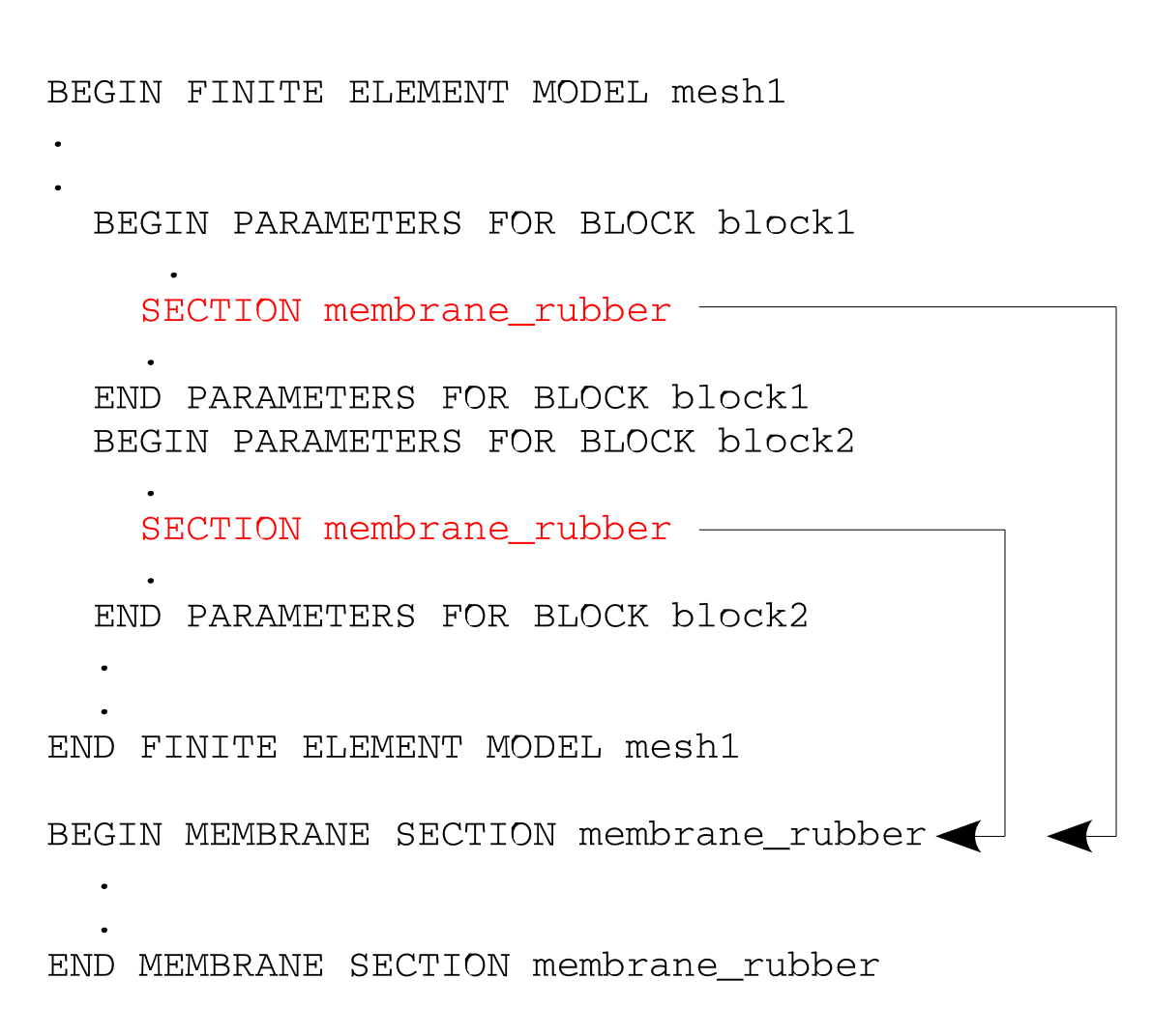
Fig. 6.1 Association between SECTION command lines and a section command block.

6.1.7.6. Linear and Quadratic Bulk Viscosity

LINEAR BULK VISCOSITY =
  <real>linear_bulk_viscosity_value(0.06)
QUADRATIC BULK VISCOSITY =
  <real>quad_bulk_viscosity_value(1.20)

The linear and quadratic bulk viscosity are set with these two command lines. Consult the documentation for the elements [[5]] for a description of the bulk viscosity parameters.

6.1.7.7. Hourglass Control

HOURGLASS STIFFNESS = <real>hourglass_stiff_value(0.05)
HOURGLASS VISCOSITY = <real>hourglass_visc_value(0.0)
MEMBRANE HOURGLASS STIFFNESS =
  <real>memb_hourglass_stiff_value(0.05)
MEMBRANE HOURGLASS VISCOSITY =
  <real>memb_glass_visc_value(0.0)
BENDING HOURGLASS STIFFNESS =
  <real>bend_hourglass_stiff_value(0.05)
BENDING HOURGLASS VISCOSITY =
  <real>bend_glass_visc_value(0.0)
TRANSVERSE SHEAR HOURGLASS STIFFNESS =
  <real>tshr_hourglass_stiff_value(0.05)
TRANSVERSE SHEAR HOURGLASS VISCOSITY =
  <real>tshr_glass_visc_value(0.0)
HOURGLASS TRANSITION STRAIN =
  <real>hourglass_transition_strain_value(1.0)
HOURGLASS EXPONENT = <real>hourglass_exponent_value(1.0)

These command lines set the hourglass control parameters for elements that use hourglass control. Currently, the included elements are the eight-node, uniform-gradient hexahedral elements; the eight-node and ten-node tetrahedral elements; and the four-node membrane and shell elements. Consult the element documentation [[5]] for a description of the hourglass parameters.

Hourglass stiffness and viscosity parameters for under integrated elements are set using the HOURGLASS STIFFNESS and HOURGLASS VISCOSITY commands, respectively. If either of these commands are used for shell elements, they set the hourglass stiffness or viscosity for all three modes (membrane, bending, and transverse shear).

Hourglass parameters for the membrane, bending, and transverse shear modes can be set individually for shell elements. The membrane hourglass stiffness and viscosity can be set with the MEMBRANE HOURGLASS STIFFNESS and MEMBRANE HOURGLASS VISCOSITY commands. These membrane hourglass commands can also be used with membrane elements. The bending hourglass stiffness and viscosity are set with the BENDING HOURGLASS STIFFNESS and BENDING HOURGLASS VISCOSITY commands, and transverse shear hourglass stiffness and viscosity are set with the TRANSVERSE SHEAR HOURGLASS STIFFNESS and TRANSVERSE SHEAR HOURGLASS VISCOSITY commands. These commands will override either the default values and any value set in the generic HOURGLASS STIFFNESS and/or HOURGLASS VISCOSITY commands for the particular mode that is specified.

The hourglass stiffness parameter defaults to 0.05 for all elements using hourglass control. The hourglass viscosity parameter defaults to 0.0 for all elements using hourglass control.

Hourglass resistances are scaled by the material effective modulus. The hourglass resistance can be strongly affected by the method that computes the effective moduli. The command line in Section 6.1.7.8 selects the method for computing the effective moduli.

The HOURGLASS TRANSITION STRAIN and HOURGLASS EXPONENT commands only apply to the HYPERELASTIC hourglass formulation. The hyperelastic hourglass is a nonlinear hourglass control formulation. The nonlinearity becomes prominent once the hourglass strain reaches the HOURGLASS TRANSITION STRAIN. The strength of the nonlinearity is controlled by the HOURGLASS EXPONENT, where the default exponent of 1.0 gives a linear hourglass force-displacement relation. For problems where the hourglass modes are highly excited, an exponent of 2.0 with a transition strain of 0.025 is recommended to mitigate the possibility of element inversion. With these settings, the hourglass stiffness increases so that the hourglass models can hold more energy in extreme deformation situations, increasing simulation robustness but perhaps reducing accuracy. See the Sierra/SM Theory Manual [[6]] for more details.

6.1.7.8. Effective Moduli Model

EFFECTIVE MODULI MODEL =
  <string>PRONTO|ELASTIC|PROBED(PRONTO/ELASTIC)

The element-based critical time step and hourglass force computations require a measure of the material moduli, which is given in Sierra/SM by the effective moduli. The CFL condition dictates that the critical time step is directly related to the current material moduli, and the hourglass forces must be appropriately scaled based on the material moduli. For elastic, isotropic material models, the moduli are constant throughout the analysis. However, for nonlinear materials, the moduli are typically computed numerically from the stresses. For models with softening regimes or that approach perfect plasticity, the moduli may be difficult to define, and the way in which they are computed may adversely affect the analysis. Through the EFFECTIVE MODULI MODEL command line, Presto provides several methods for the computation of these effective moduli:

• PRONTO This method is the default when running an explicit calculation and is identical to the method of computing effective moduli present in the Pronto3D code. This method will compute an approximate tangent modulus based on current material response. The PRONTO method includes some bounds on admissible tangent stiffness values to promote stability. The PRONTO method can produce poor results in analyses with materials that undergo substantial hardening; the PROBED modulus may be a better option for such materials.

• PROBED This method calls the material stiffness calculations twice each step to compute a true tangent probe of the material stiffness. It is generally more accurate and robust than the PRONTO method, although more expensive, as it requires two rather than one material call per time step. The PROBED option may be worth using for models were the material stiffness changes greatly (such as compressible foams). Note the probe modulus is a probe of the instantaneous tangent modulus and may have difficulty taking in to the account of rate-dependent effects such as creep or strain rate hardening.

• MATERIAL A handful of material models are able to compute an analytic tangent stiffness. Currently this includes only the HYPER FOAM and the MOONEY RIVLIN material models. When the analytic result is available it provides the most robust and most efficient estimate of the tangent stiffness. The PRONTO and PROBED methods will both use the analytic tangent modulus if possible and revert to a numerical tangent calculation for materials that do not compute an analytic tangent modulus.

• ELASTIC This method uses the initial elastic moduli for the entire analysis. For materials that harden substantially (such as compressible foams) the elastic method could produce moduli late in the analysis that are too low causing stability problems. For materials the have constant stiffness or if the elastic constants are set in a way to be conservative for the entire analysis routine the elastic modulus method may be the most robust. The elastic modulus is the default method when running an implicit calculation.

The EFFECTIVE MODULI MODEL command line should be used with caution because it can strongly affect the analysis results.

The commands

• MINIMUM EFFECTIVE DILATATIONAL MODULI RATIO and

• MINIMUM EFFECTIVE SHEAR MODULI RATIO

define the minimum effective modulus that can be computed for a material with respect to the initial elastic modulus. This value prevents the computed tangent modulus from dropping to close to zero for yielding or softening materials. A larger value for this constant can sometimes promote stability by allowing the effective modulus to track with material stiffness, but not bottom out at such a low value that low stiffness instability can occur. The computed effective dilatational modulus value primarily affects timestep and bulk viscosity calculations (which can affect the speed of elastic wave propagation). The computed effective shear modulus primarily affects hourglass control in the elements. For historical reasons the default value for these parameters depends on the effective moduli model used; the default ratios are listed in Table Table 6.1.

Table 6.1 Default moduli ratios for the various effective moduli models.

Model	Dilatational ratio	Shear ratio
PRONTO	\(0.001\)	\(0.05\)
PROBED	\(1.0\mathrm{e}{-6}\)	\(1.0\mathrm{e}{-6}\)
ELASTIC	\(1.0\)	\(1.0\)

6.1.7.9. Activation/Deactivation of Element Blocks by Time

ACTIVE FOR PROCEDURE <string>proc_name DURING PERIODS
  <string list>period_names
INACTIVE FOR PROCEDURE <string>proc_name DURING PERIODS
  <string list>period_names

This command line permits the activation and deactivation of element blocks by time period. The time periods are defined in the TIME STEPPING BLOCK command block (Section 3.1.1) within a specific procedure named in a PRESTO PROCEDURE or an ADAGIO PROCEDURE command block (Section 2.2).

The ACTIVE FOR PROCEDURE or INACTIVE FOR PROCEDURE command lines can optionally be used to deactivate element blocks for a portion of the analysis. If the ACTIVE FOR PROCEDURE command is used, the element block is active for all periods listed for the named procedure, and is deactivated for all time periods that are absent from the list. If the INACTIVE FOR PROCEDURE command is used, the element block is deactivated for all periods listed for the named procedure. The element block is active for all time periods that are absent from the list. If neither command line is used, by default the block is active during all time periods. This command line controls the activation and deactivation of all elements in a block. Alternatively, individual elements can be deactivated with the ELEMENT DEATH command block (see Section 6.5).

Warning

Inactive element’s corresponding nodes will not move while they are inactive except when the nodes are shared with active elements. It is therefore possible that inactive elements can be inverted while inactive and trigger a fatal error when activated.

Known Issue

Deactivation of element blocks does not currently work in conjunction with the full tangent preconditioner (see Section 4.3) in Adagio. To use this capability, one of the nodal preconditioners must be used.

Known Issue

Deactivating a block only turns off the element/material computations and does not remove the blocks degrees of freedom from the solution matrix. Thus if the nodes have some external force applied convergence may be impossible in implicit or the nodes may accelerate to infinite velocity in explicit. It is recommended that on time periods that a block is deactivated a kinematic boundary condition that fixes all degrees of freedom of the deactivated block also be used.

6.1.8. Element Block Default Parameters

BEGIN BLOCK DEFAULTS
  MATERIAL = <string>material_name
  MODEL    = <string>model_name
  SECTION  = <string>section_id
  LINEAR BULK VISCOSITY =
    <real>linear_bulk_viscosity_value(0.06)
  QUADRATIC BULK VISCOSITY =
    <real>quad_bulk_viscosity_value(1.20)
  HOURGLASS STIFFNESS =
    <real>hourglass_stiff_value(0.05)
  HOURGLASS VISCOSITY =
  <real>hourglass_visc_value(0.0)
  EFFECTIVE MODULI MODEL =
    <string>PRONTO|ELASTIC|PROBED(PRONTO/ELASTIC)
  MINIMUM EFFECTIVE SHEAR MODULI RATIO =
    <real>min_eff_mod_ratio
  MINIMUM EFFECTIVE DILATATIONAL MODULI RATIO =
    <real>min_eff_mod_ratio
END [BLOCK DEFAULTS]

The block defaults block may be used modify the default values for commands used inside the BEGIN PARAMETERS FOR BLOCK blocks within the same BEGIN FINITE ELEMENT MODEL command block. See section Section 6.1.7 for the description of each command.

Block defaults can be used to simplify input when a model has a large number of blocks. For example to try an alternative effective moduli method or hourglass stiffness at all blocks at once. If a given parameter is set in both block defaults and a specific block the specific block value overrides the block default value. The following examples demonstrate use of the block defaults command.

Example 1:

begin block defaults
  hourglass stiffness = 0.10
  hourglass viscosity = 0.01
end
begin parameters for block block_1
  material = steel
  model    = elastic
end
begin parameters for block block_2
  material = rubber
  model    = mooney_rivlin
end

In this example the hourglass stiffness and viscosity defaults have been changed for all blocks. This would be equivalent to the following input:

begin parameters for block block_1
  material = steel
  model    = elastic
  hourglass stiffness = 0.10
  hourglass viscosity = 0.01
end
begin parameters for block block_2
  material = rubber
  model    = mooney_rivlin
  hourglass stiffness = 0.10
  hourglass viscosity = 0.01
end

Example 2:

begin block defaults
  material = aluminum
  model    = elastic_plastic
  section  = solid_1
end
begin parameters for block block_1
end
begin parameters for block block_2
end
begin parameters for block block_3
end
begin parameters for block block_4
  material = tungsten
  model    = elastic
end

A default material is used for blocks one two and three, but the defaults are partially overridden for block 4. This would be equivalent to the following input:

begin parameters for block block_1 block_2 block_3
  material = aluminum
  model    = elastic_plastic
  section  = solid_1
end
begin parameters for block block_4
  material = tungsten
  model    = elastic
  section  = solid_1
end

6.1.9. Create Assemblies

BEGIN ASSEMBLY <string>assembly_name
  NODESET = <string list>nodelist_names
  SURFACE = <string list>surface_names
  BLOCK = <string list>block_names
  ASSEMBLY = <string list>assembly_names
  NODESET_ID LIST = <integer list> nodeset_integerIDs
  SURFACE_ID LIST = <integer list> surface_integerIDs
  BLOCK_ID LIST = <integer list> block_integerIDs
  ALLOW MISSING BLOCK IDS = OFF|ON (OFF)
END ASSEMBLY [<string>assembly_name]

The BEGIN ASSEMBLY command block allows the user to create assemblies, which are groups of mesh objects. Assemblies may consist of element blocks, surfaces, node sets, or other assemblies. They are permitted to contain only one type of mesh entity. However, an assembly may be composed of assemblies with different entity types. For example, an assembly could be made of an assembly of element blocks and an assembly of surfaces.

The prescription of some boundary conditions is limited to certain mesh entity types. This places restrictions on the mesh entity types that an assembly may contain for these boundary conditions. For example, if a boundary condition may only be specified for an element block, a specified assembly may only contain element blocks.

Assemblies are intended to streamline input files significantly by enabling the user to specify boundary conditions to groups of mesh objects at once. This can make a big difference in the input files of especially large models.

In the command block, assembly_name is the name given to the assembly. The assembly name cannot be identical to that of another block, surface, or nodeset. The command lines that follow are used to specify the mesh entities that make up the assembly. While assemblies may be added to assemblies only by name, node sets, surfaces, or element blocks may be added to assemblies by name, or by integer identifier (integerID). The identifiers may be specified as a list of integers, or as a range in one of two formats: FirstID:LastID:Increment, or FirstID:LastID, which assumes the increment is 1. One of NODESET, SURFACE, BLOCK, ASSEMBLY, NODESET_ID LIST, SURFACE_ID LIST, or BLOCK_ID LIST is required to be listed. Blocks, surfaces, or nodesets may be a part of more than one assembly. If an assembly already exists on the input mesh or as a previous assembly, defining it again will result in modifying the assembly so that it contains the union of the entities in the original and the new instance.

For example, a prescribed force can be specified for a series of blocks as:

begin prescribed force
   block = block_1 block_2 block_3 block_4 block_5
   component = x
   function = sierra_constant_function_one
   scale factor = 1000
end

With assemblies, this can be specified as:

begin prescribed force
   assembly = assembly_1
   component = x
   function = sierra_constant_function_one
   scale factor = 1000
end

where assembly_1 consists of block_1, block_2, block_3, block_4, and block_5.

This assembly would be defined in the Finite Element Model part of the input file as:

begin assembly assembly_1
   block = block_1 block_2 block_3 block_4 block_5
end assembly

The blocks in the assembly may be listed in separate line commands:

begin assembly assembly_1
   block = block_1
   block = block_2
   block = block_3
   block = block_4
   block = block_5
end assembly

Alternatively, the blocks’ integer identifiers may be specified as a list in one of three formats to create the assembly. One approach is to use the ID ranges with incrementation:

begin assembly assembly_1
   block_id list = 1:5:1
end assembly

Since the increment in IDs is 1, the increment may be omitted:

begin assembly assembly_1
   block_id list = 1:5
end assembly

The individual integer identifiers may also be listed:

begin assembly assembly_1
   block_id list = 1 2 3 4 5
end assembly

If an assembly is already present in the input mesh, the user may add additional mesh entities to the existing assembly. For example, if assembly_1 exists on the input mesh and consists of block_1, block_2, and block_3, it can be expanded to include block_4 and block_5 by adding the following to the input file:

begin assembly assembly_1
   block = block_4 block_5
end assembly

When mesh assemblies are modified in this way the logfile outputs a warning alerting the user of the operation.

The command ALLOW MISSING BLOCK IDS will let the user set any block id in BLOCK_ID LIST even if they don’t exist. Missing ids will be silently ignored when this command is on.

begin assembly assembly_1
   block_id list = 1:100 # only 5 blocks exist in the mesh
   allow missing block ids = on
end assembly

---

[1] (1,2,3,4)

L.M. Taylor and D.P. Flanagan. Pronto3D: a three-dimensional transient solid dynamics program. Technical Report SAND87-1912, Sandia National Laboratories, Albuquerque, NM, March 1989. URL: http://infoserve.sandia.gov/sand_doc/1987/871912.pdf.

[2] (1,2,3)

M.M. Rashid. Incremental kinematics for finite element applications. International Journal for Numerical Methods in Engineering, 36:3937–3956, 1993. doi:10.1002/nme.1620362302.

[3]

C.R. Dohrman, M.W. Heinstein, J. Jung, S.W. Key, and W.R. Witkowski. Node-based uniform strain elements for three-node triangular and four-node tetrahedral meshes. International Journal for Numerical Methods in Engineering, 47:1549–1568, 2000. doi:10.1002/(SICI)1097-0207(20000330)47:9<1549::AID-NME842>3.0.CO;2-K.

[4] (1,2)

S.W. Key and C.C. Hoff. An improved constant membrane and bending stress shell element for explicit transient dynamics. Computer Methods in Applied Mechanics and Engineering, 124(1–2):33–47, 1995. doi:10.1016/0045-7825(95)00785-Y.

[5] (1,2)

T.A. Laursen, S.W. Attaway, and R.I. Zadoks. SEACAS theory manuals: part III. finite element analysis in nonlinear solid mechanics. Technical Report SAND98-1760/3, Sandia National Laboratories, Albuquerque, NM, 1999. URL: http://infoserve.sandia.gov/sand_doc/1998/981760-3.pdf.

[6]

Sierra/SolidMechanics Team. Sierra/SolidMechanics VOTD Theory Manual. Technical Report In draft, Sandia National Laboratories, Albuquerque, NM, 2019.