8.5. Friction Models

Friction models are used to describe the physics of interactions that occur between contact surfaces. The user then associates these friction models to pairs of surfaces in the interaction-definition blocks (see Section 8.6.1 and Section 8.6.2). During the search phase of contact, node-face or face-face interactions are identified, and the designated friction model is used to determine how the resulting contact forces are resolved between these surface pairs.

Not all friction models are available with all analysis types and all contact libraries. If a model is not available for certain analysis types, that fact is noted in the documentation of those models below.

In addition to the friction models, any of the cohesive zone models available for use with interface elements (see Section 5.3) can be used as interface models within explicit dynamic analyses. See Section 8.6.2.4 for more details on the usage of those models within contact.

All friction models are command blocks, although some of the models do not have any command lines inside the command block. The commands for defining the available friction models are described next. Friction models are associated with specific pairings of contact surfaces through the interaction-definition blocks in Section 8.6.1 and Section 8.6.2.

By default, interactions between contact surfaces with no friction model assigned are treated as frictionless.

8.5.1. Frictionless Model

BEGIN FRICTIONLESS MODEL <string>name
END [FRICTIONLESS MODEL <string>name]

The FRICTIONLESS MODEL command block defines frictionless contact between surfaces. In frictionless contact, contact forces are computed normal to the contact surfaces to prevent penetration, but no forces are computed tangential to the contact surfaces. The string name is a user-selected name for this friction model that is used when identifying this model in the interaction definitions. No command lines are needed inside the command block. A default named frictionless model named frictionless can be used without defining this command block.

8.5.2. Constant Friction Model

BEGIN CONSTANT FRICTION MODEL <string>name
  FRICTION COEFFICIENT = <real>coeff
END [CONSTANT FRICTION MODEL <string>name]

The CONSTANT FRICTION MODEL command block defines a constant coulomb friction coefficient between two surfaces as they slide past each other in contact. No resistance is provided to keep the surfaces together if they start to separate. The string name is a user-selected name for this friction model that is used to identify this model in the interaction definitions, and coeff is the constant coulomb friction coefficient. There is no default value for the friction coefficient.

8.5.3. Velocity Dependent Coulomb Friction Model

BEGIN VELOCITY DEPENDENT COULOMB MODEL <string>name
  COULOMB COEFFICIENT = <string>coeff_func
END [VELOCITY DEPENDENT COULOMB MODEL <string>name]

The VELOCITY DEPENDENT COULOMB MODEL command block defines a Coulomb friction law between two surfaces as they slide past each other in contact. The value of the Coulomb coefficient at any given time is a function of the relative velocity at the interface. No resistance is provided to keep the surfaces together if they start to separate. The string name is a user-selected name for this friction model that is used to identify this model in the interaction definitions. The COULOMB COEFFICIENT command provides coeff_func, the name of a previously defined XY function, where X is the velocity magnitude and Y is the coulomb coefficient. The velocity dependent coulomb model can be used to define stick-slip friction behavior where the friction coefficient is the stick value when velocity is nominally small and the slip value when velocity is larger than some nominal value.

8.5.4. Variable Coefficient Coulomb Model

BEGIN VARIABLE COEFFICIENT COULOMB MODEL <string>name
  FUNCTION ARGUMENT: <name> = SIDE A NODAL <var_name>
  FUNCTION ARGUMENT: <name> = SIDE B  NODAL <var_name>
  COEFFICIENT FUNCTION      = <string>coeff_func
END VARIABLE COEFFICIENT COULOMB MODEL <string>name

The VARIABLE COEFFICIENT COULOMB MODEL command block can be used to define a Coulomb friction law where the friction coefficient is dependent on some arbitrary nodal variable. For example, a different coefficient based on spatial coordinates or from some surface dependent property. See Section 2.1.5 for more informationon generalized functions. An example of using this friction model to compute a friction model that depends on an oxidation state nodal surface variable follows.

#
#  Friction coefficient based on oxide state. Assume
#  oxide thickness < 1.0e-6 means "clean" surface
#  and thickness > 1.0e-6 is a rough oxidized surface.
#  Friction coefficient is then subject to following rules:
#
#  oxide against oxide: u = 0.4
#  oxide against clean: u = 0.2
#  clean against clean: u = 0.1
#
begin function oxide_fric_coeff
  type is analytic
  expression variable: ox1
  expression variable: ox2
  evaluate expression = "    \#
    (ox1 < 1.0e-6) ? (       \#
      (ox2 < 1.0e-6) ? (     \#
        0.1                  \#
      ) : (                  \#
        0.2                  \#
      )                      \#
    ) : (                    \#
      (ox2 < 1.0e-6) ? (     \#
        0.2                  \#
      ) : (                  \#
        0.4                  \#
      )                      \#
    )                        \#
  "
end

begin variable coefficient coulomb model oxide_fric
  coefficient function = oxide_fric_coeff
  Function Argument: ox1 = side A nodal oxide_thick
  Function Argument: ox2 = side B  nodal oxide_thick
end

8.5.5. Tied Model

BEGIN TIED MODEL <string>name
  USE OFFSET REMOVAL = ON | OFF (OFF)
END [TIED MODEL <string>name]

The TIED friction model attaches together surfaces that are close in the initial model geometry. Tied faces will stay attached throughout the analysis. The string name is a user-selected name for this friction model that is used to identify this model in the interaction definitions. No command lines are needed inside the command block. A default tied model named tied can be used without defining this command block.

When using a tied contact friction model USE OFFSET REMOVAL = ON will remove all offset that is remaining between the tied surfaces after overlap removal.

Warning

USE OFFSET REMOVAL must be used in conjunction with BEGIN OVERLAP REMOVAL for offset to be removed.

8.5.6. Inactive Friction Model

BEGIN INACTIVE FRICTION MODEL <string>name
END [INACTIVE FRICTION MODEL <string>name]

The INACTIVE FRICTION MODEL command block specifies that the interacting surfaces product no force and contact is effectively ignored on the interaction pair. The inactive friction model can be used to selectively turn off interaction pairs. One common use is integrating the inactive friction model to a TIME VARIANT friction model to turn contact interactions off selectively by time period.

8.5.7. Dynamic Tied Model

BEGIN DYNAMIC TIED MODEL <string>name
END [DYNAMIC TIED MODEL <string>name]

The DYNAMIC TIED MODEL command block defines a contact interaction that constrains opposing faces to stay in the same relative location to each other throughout the analysis. No command lines are needed within this command block. A default dynamic tied model named dynamic_tied can be used without defining this command block. The dynamic tied model is similar to the tied model except that the dynamic tied model enforces zero relative velocity at the interface while the tied model enforces zero relative displacement. In the limit, both of these models are identical. If the analysis involves substantial topology changes, such as element death, the dynamic tied model may be more stable, but slightly less accurate.

8.5.8. Glued Model

BEGIN GLUED MODEL <string>name
END [GLUED MODEL <string>name]

Note, this model is available for explicit and implicit analyses. For implicit analyses, it can only be used with augmented Lagrange enforcement.

The GLUED model defines a contact interaction that allows the interacting faces to move independently until they come into contact, at which point they become permanently attached together. Once attached the faces can have no relative normal or tangential motion for the rest of the analysis. The string name is a user-specified name for this friction model that is used to reference this model in the interaction definitions. No command lines are needed inside the command block. A default glued model named glued can be used without defining this command block. The glued model is enforced via a zero-velocity constraint.

Warning

Because glued contact is set up using the predicted configuration during an implicit simulation the loadstep must be turned off by setting the loadstep predictor to:

begin loadstep predictor\newline
  type = scale\_factor\newline
  scale factor = 0 0\newline
end loadstep predictor

8.5.9. Glued Normal Model

BEGIN GLUED NORMAL MODEL <string>name
END [GLUED NORMAL MODEL <string>name]

The GLUED NORMAL model defines a contact interaction that allows the interacting faces to move independently until they come into contact, but once they come into contact they become permanently attached together, but are allowed to slide along each other. Once attached the faces can have no relative normal motion for the rest of the analysis. The string name is a user-specified name for this friction model that is used to reference this model in the interaction definitions. No command lines are needed inside the command block.

Warning

Because glued normal contact is set up using the predicted configuration during an implicit simulation the loadstep must be turned off by setting the loadstep predictor to:

begin loadstep predictor\newline
  type = scale\_factor\newline
  scale factor = 0 0\newline
end loadstep predictor

8.5.10. Cohesive Zone Model

BEGIN COHESIVE ZONE MODEL <string>name
  TRACTION DISPLACEMENT FUNCTION = <string>func_name
  TRACTION DISPLACEMENT SCALE FACTOR = <real>scale_factor(1.0)
  CRITICAL NORMAL GAP = <real>crit_norm_gap
  CRITICAL TANGENTIAL GAP = <real>crit_tangential_gap
END [COHESIVE ZONE MODEL <string>name]

The COHESIVE ZONE MODEL command block defines a friction model that prevents penetration when contact surfaces are touching, and provides an additional force when the distance between the node and face in an interaction increases. This force is determined by a user-specified function. Once the distance exceeds a user-specified value in the normal direction or the tangential direction, the force is no longer applied. This model can be used to simulate the energy required to separate two surfaces that are initially touching.

In the above command block, the string name is a user-selected name for this friction model that is used to identify this model in the interaction definitions. The traction-separation relationship is given by the TRACTION DISPLACEMENT FUNCTION command line, where the string func_name is the name of a function defined in a FUNCTION command block in the SIERRA scope. The \(y\)-values of this function can be scaled by the real value scale_factor in the TRACTION DISPLACEMENT SCALE FACTOR command line; the default for this factor is 1.0. In the CRITICAL NORMAL GAP command line, the real value crit_norm_gap specifies the normal distance between the node and face past which the cohesive zone no longer provides a force. Similarly, in the CRITICAL TANGENTIAL GAP command line, the real value crit_tangential_gap specifies the tangential distance between the node and face past which the cohesive zone no longer provides a force.

The function referenced by the TRACTION DISPLACEMENT FUNCTION command line must be an XY function (see Section 2.1.5). The X-values correspond to \(\epsilon\), defined as:

\[\epsilon=\frac{current\ displacement}{critical\ gap\ length}\]

\(\epsilon\) is a non-dimensional quantity which should start at zero corresponding to zero traction, and end at 1.0 corresponding to the critical gap length. The Y-values are the \(\epsilon\)-dependent tractions between faces sharing a cohesive zone. All traction and separation quantities should be positive.

The following example is the problem shown in Fig. 8.12: 2 bricks being pulled apart that are initially connected by a cohesive zone.

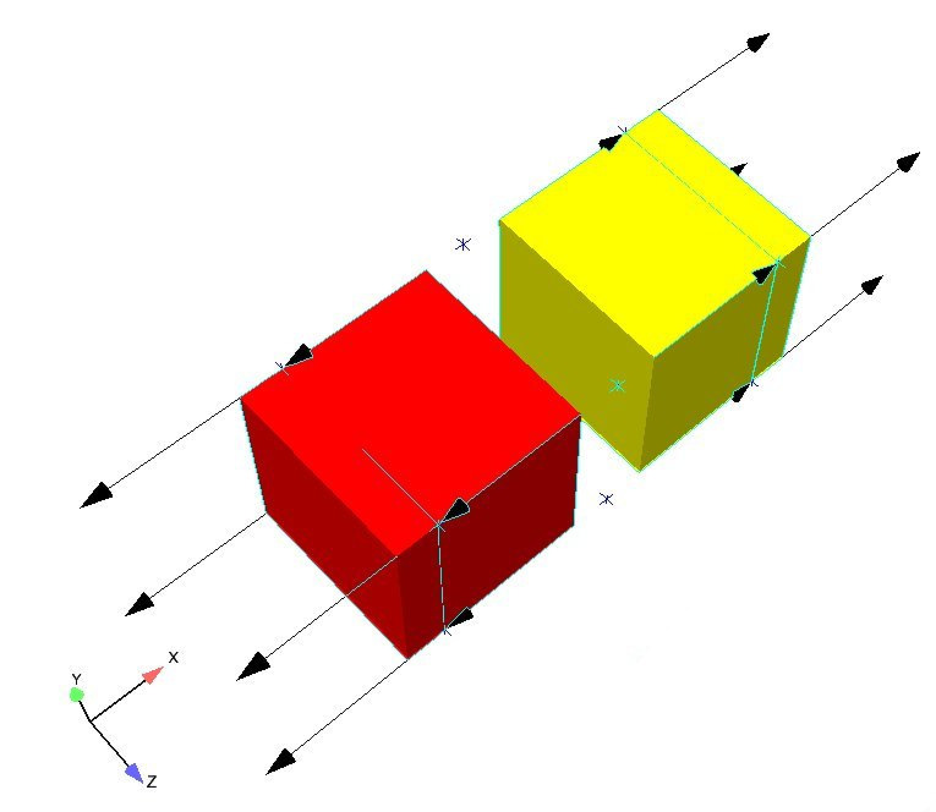
Fig. 8.12 Bricks sharing a cohesive zone and being pulled apart.

The function describing the cohesive zone is given by:

begin function spring_restore
  type = piecewise linear
  begin values
    # separation(epsilon) traction
    0.0   0.0
    0.1   1.0
    0.3   9.0
    0.4  16.0
    0.5  25.0
    0.9  81.0
    1.0 100.0
  end values
end function spring_restore

The cohesive zone model is given by:

begin cohesive zone model cohesive_zone
  critical normal gap = 0.05
  critical tangential gap = 0.05
  traction displacement function = spring_restore
  traction displacement scale factor = 2.5E+02
end cohesive zone model cohesive_zone

A plot of the \(x\)-displacement for node 8 (one of the nodes on the cohesive zone) over time is given in Fig. 8.13. The corresponding cohesive force in the \(x\)-direction over time for node 8 is shown in Fig. 8.14.

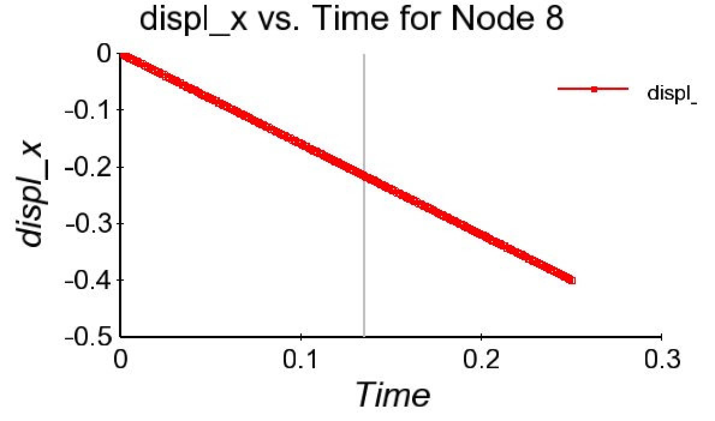
Fig. 8.13 Displacement X vs. time for node 8.

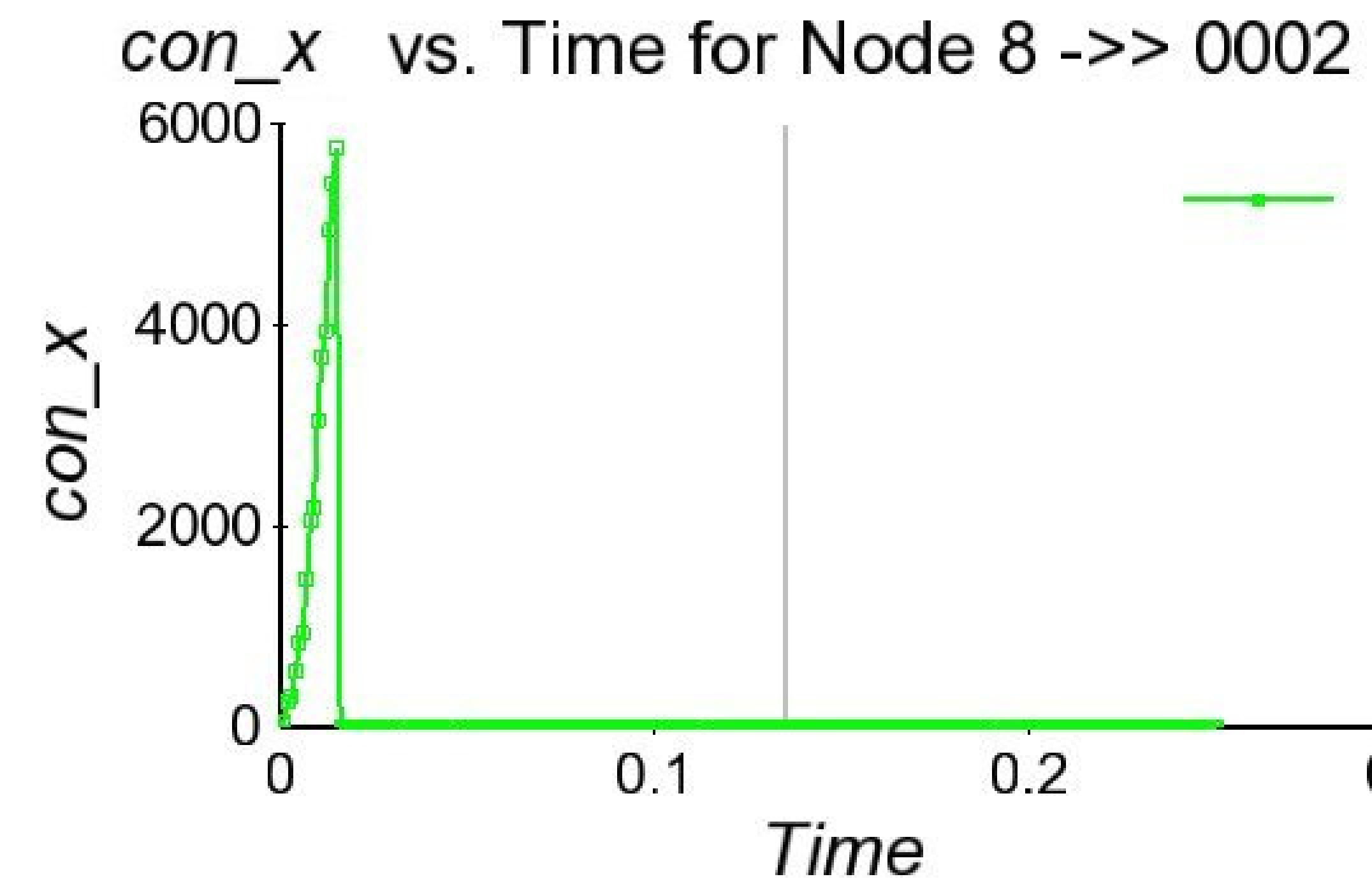
Fig. 8.14 Cohesive force in x vs. time for node 8.

As expected, when the displacement exceeds the critical normal gap of .05, which happens at .016 seconds, the cohesive force goes to zero. The cohesive zone force peaks at 6250, which is equal to:

\[\frac{force\ at\ critical\ gap \times traction\ displacement\ scale\ factor}{number\ of\ nodes\ on\ face} = \frac{100 \times 250}{4}.\]

8.5.11. Hybrid Model

BEGIN HYBRID MODEL <string>name
  INITIALLY CLOSE = <string>close_name
  INITIALLY FAR   = <string>far_name
END [HYBRID MODEL <string>name]

The HYBRID MODEL command block defines a single friction model that is a composite of two other models: one for faces that are initially close together, and one for faces that are initially far apart. The friction law specified in the INITIALLY CLOSE command is used for faces that are close together in the initial mesh geometry. The friction law specified in the INITIALLY FAR command is used for faces that are far apart in the initial mesh geometry.

A common usage of the hybrid model is to tie together parts of two surfaces that are close together, while allowing the remaining parts of those surfaces to have a sliding contact interaction. If the tied model were used in that situation, the faces that are initially close would be tied together, but no contact would be enforced on the remaining faces on those surfaces, so they could pass through one another. Another potential usage of the hybrid model would be to define a high friction coefficient for faces that are initially close, and then use a lower friction coefficient once the faces start to slide away from the initial configuration.

A hybrid model is automatically created when an interaction-specific and a default friction model are both specified and the interaction-specific friction law is only applicable when the surfaces are initially close together. For example, the hybrid model contact interaction definition:

BEGIN HYBRID MODEL hmod
  INITIALLY CLOSE = tied
  INITIALLY FAR   = frictionless
END

BEGIN INTERACTION
  SURFACES = block_1 block_2
  friction model = hmod
END

Is equivalent to:

BEGIN INTERACTION DEFAULTS
  FRICTION MODEL = frictionless
END
BEGIN INTERACTION
  SURFACES = block_1 block_2
  friction model = tied
END

The hybrid model definition above was used for the example model shown in Fig. 8.15.

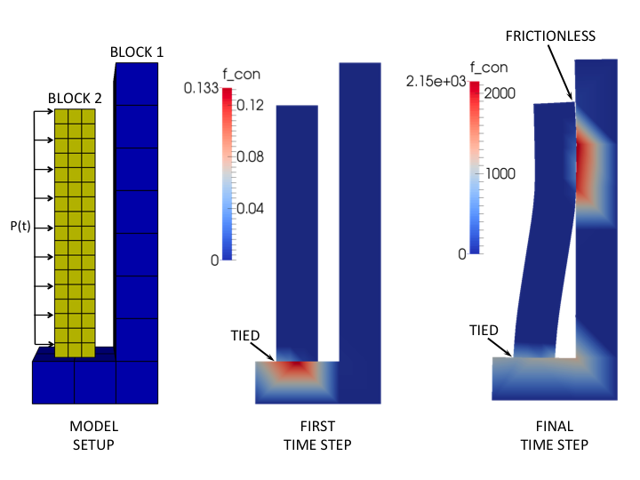
Fig. 8.15 Example usage of the hybrid friction model. The contour plots show the magnitude of the contact force.

Warning

Using the hybrid friction model may cause your simulation to have poor performance. This is especially the case when you have a large number of element blocks.

8.5.12. Time Variant Model

BEGIN TIME VARIANT MODEL <string>name
  MODEL = <string>model DURING PERIODS <string list>time_periods
END [TIME VARIANT MODEL]

Note: This feature is only available for Dash contact with explicit dynamics and Dash augmented Lagrange contact for implicit analyses.

The TIME VARIANT MODEL command block does not directly define a friction model, but provides a mechanism to switch between separately defined friction models between time periods. The only command line in the block is the MODEL command, which is used to reference a separately-defined friction model model and provide a list of time periods during which that model is active. Multiple MODEL commands may be used to activate different friction models throughout the analysis. See Section 2.6 for more information on controlling functionality by time period.

Warning

Using the time variant friction model may cause your simulation to have poor performance. This is especially the case when you have a large number of element blocks.}

8.5.13. Nodal Field Dependent Model

BEGIN NODAL FIELD DEPENDENT FRICTION MODEL <string>name
  INITIAL CONTACT TRANSITION VALUE = <real>transition_value
  CONTACT TRANSITION REDUCTION METHOD =
    <string>MIN|MAX|INTERPOLATE(MAX)
END [NODAL FIELD DEPENDENT FRICTION MODEL]

Note: This feature is only available for Dash contact with explicit dynamics and Dash augmented Lagrange contact for implicit analyses.

The NODAL FIELD DEPENDENT FRICTION MODEL command block allows the opportunity to vary the friction coefficient and switch between Coulomb and glued friction conditions based on the value of a specific nodal variable, named contact_transition. For every interaction pair for which this friction model is applied, the contact_transition field is evaluated on the side B nodes to determine the type of contact: a non-negative contact_transition value results in Coulomb contact and a negative value results in glued contact. For Coulomb contact, the coefficient of friction is set equal to the contact_transition value.

The contact_transition field is controlled by the user. The input command INITIAL CONTACT TRANSITION VALUE sets an initial value for all nodes in the model. The field can then be varied spatially and temporally by a USER OUTPUT command block (Section 9.4), where contact_transition is the variable name. This allows the user to define contact_transition as a function of other field variables. For example, the following input commands make the contact conditions dependent on the temperature of element block block_1:

BEGIN FUNCTION my_temperature
  TYPE IS PIECEWISE ANALYTIC
  BEGIN EXPRESSIONS
    # time  temperature
    0.0     "600.0"
    0.00006 "600.0+1400.0*(x-0.00006)/0.00394"
    0.004   "2000.0-1600.0*(x-0.004)/0.0005"
    0.0045  "400.0"
  END
END FUNCTION my_temperature

BEGIN FUNCTION temp_dependent_fric
  TYPE IS ANALYTIC
  EXPRESSION VARIABLE: q = GLOBAL temperature_max
  EVALUATE EXPRESSION IS "q > 500.0 ? (2000.0-q)/4000.0 : -1.0"
END FUNCTION temp_dependent_fric

BEGIN PRESCRIBED TEMPERATURE
  BLOCK = block_1
  FUNCTION = my_temperature
END PRESCRIBED TEMPERATURE

BEGIN USER OUTPUT
  BLOCK = block_1
  COMPUTE GLOBAL temperature_max AS MAX OF NODAL temperature
END USER OUTPUT

BEGIN USER OUTPUT
  BLOCK = block_1 block_2
  COMPUTE NODAL contact_transition AS FUNCTION temp_dependent_fric
END USER OUTPUT

BEGIN CONTACT DEFINITION slide_and_glued
  SEARCH = DASH
  SKIN ALL BLOCKS = ON

  BEGIN INTERACTION
    SURFACES = block_1 block_2
    FRICTION MODEL = temperature_dependent
  END INTERACTION

  BEGIN NODAL FIELD DEPENDENT FRICTION MODEL temperature_dependent
    INITIAL CONTACT TRANSITION VALUE = 0.35
    CONTACT TRANSITION REDUCTION METHOD = MAX
  END NODAL FIELD DEPENDENT FRICTION MODEL temperature_dependent
END CONTACT DEFINITION slide_and_glued

In this example, the friction conditions are Coulomb at above 500.0 degrees and glued at 500.0 degrees or less. Above 500.0 degrees, the friction coefficient varies linearly with temperature. The temperature of block_1 starts out above 500.0 degrees and varies significantly causing a variation in the friction coefficient, until a time just prior to 0.0045 when the friction conditions become glued. The temperature of block_1 is stored as the global variable temperature_max so that both blocks involved in the interaction, block_1 and block_2, will have the correct contact_transition value, which is computed by calling the temperature_dependent_friction function in a USER OUTPUT command block. By default, the Dash algorithms internally determine the side A and side B surfaces of a contact interaction, so it is necessary to set the contact_transition field to the desired values on both surfaces involved in the interaction.

The input command CONTACT TRANSITION REDUCTION METHOD defines how the nodal contact_transition field is reduced to a single scalar at the point of interaction inside a face. The MIN and MAX options take the minimum and maximum, respectively, of the face’s nodal values. The INTERPOLATE option interpolates the nodal values to the point of interaction.