8.1. Overview of Contact Constraints

Contact between surfaces is modeled by first defining and then enforcing a set of contact constraints. A simple example of contact is shown in Fig. 8.1(a). Block \(a\) has exterior surface \(a\), and block \(b\) has exterior surface \(b\), each defined by a collection of finite element faces. For this two-dimensional drawing, the faces are straight lines between two nodes.

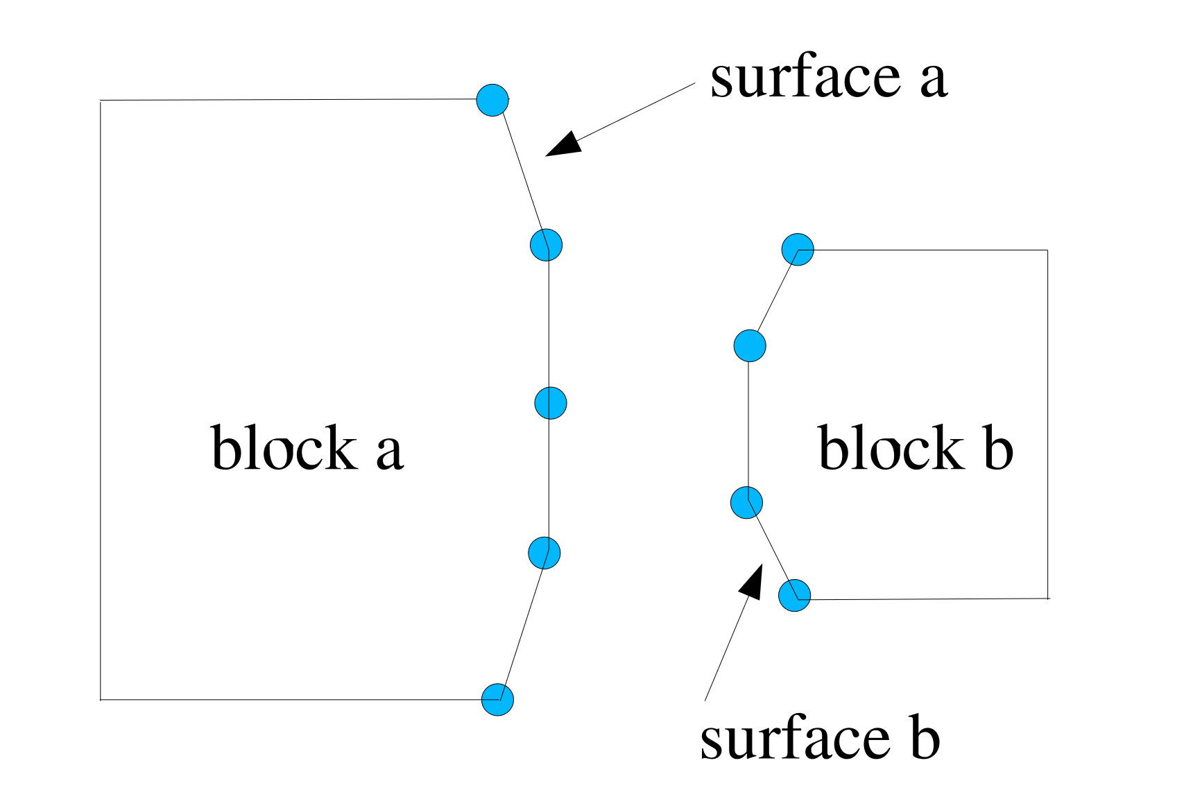(a) Time step n before contact.

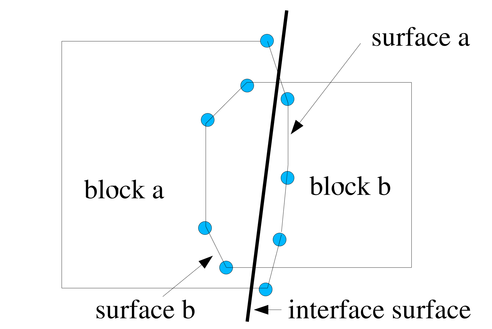(b) Time step n+1 after penetration.

Fig. 8.1 Two blocks in contact.

Fig. 8.1(a) shows the two blocks at time step \(n\). Fig. 8.1(b) shows the blocks at time step \(n+1\) when the blocks have moved and deformed under the influence of external and internal forces. Before contact is taken into account, the two blocks interpenetrate one another. This initial, potentially interpenetrated configuration is known as the initial predicted configuration. The interpenetration is removed by applying the contact algorithm.

There are three major types of contact constraints available in Sierra/SM. Node/face contact constraints are based on the concept of preventing nodes from penetrating faces on the opposing surface. Face/face constraints prevent faces on opposing surfaces from penetrating each other. Node/analytic surface constraints prevent nodes from penetrating analytically defined surfaces.

For node/face constraints, interpenetration occurs as shown in Fig. 8.1(b) when any node on surface \(a\) passes through a face of surface \(b\) or a node on surface \(b\) passes through a face of surface \(a\). One option to remove interpenetration would be to force all the nodes on surface \(a\) to lie on surface \(b\), where surface \(b\) has the configuration shown in Fig. 8.1(b). In this case, surface \(b\) would be the side A surface and surface \(a\) would be the side B surface. Alternatively, all nodes on surface \(b\) could be forced to lie on surface \(a\), in which case surface \(a\) is the side A surface and surface \(b\) is the side B. It is generally best to let the code decide the side A and side B surfaces, but the specific designations can also be input by the user.

More typically, nodes on both surfaces are moved to what can be described as an interface surface, which is shown by a thick black line in Fig. 8.1(b). The interface surface shown here as a straight line could be curved in reality. For each node on surface \(a\) that has penetrated a face on surface \(b\), forces based on the amount of node penetration are placed on both the node on \(a\) and the nodes associated with the face on \(b\). Likewise, forces are computed for each node on surface \(b\) that has penetrated some face on surface \(a\) and for the nodes associated with the penetrated face on surface \(a\). The combination of all these forces will remove the interpenetration of the two blocks and produce the final interface configuration.

The preceding two-dimensional example is analogous to much of the contact that is encountered when contact is used in an analysis. Surfaces are generated that consist of a collection of faces. Contact interactions consisting of node-face pairs are defined on the current geometry and then contact enforcement is used to remove the interpenetration of the surfaces and satisfy surface physics.