13.2. B. Implicit Quasistatic Example Problem
This appendix provides an example problem to illustrate the construction of an input file for an analysis. The problem is modeled after a pencil/eraser that is pressed against and rubbed across a tablet. The pencil, eraser and tablet are represented by blocks 1, 2 and 3 respectively. Block 4 is used to apply kinematics directly to the eraser via tied contact between block 4 and block 2. Block 1 is superfluous except when viewed together with blocks 1, 2 and 3. Then they closely resemble a pencil with an eraser on a tablet. The problem demonstrates the overall structure of an input file and includes the use of both tied and frictional contact simultaneously, the multilevel solver, and a linear solver for preconditioning. A schematic of the problem is shown in Fig. 13.3 and the mesh is shown in Fig. 13.4.
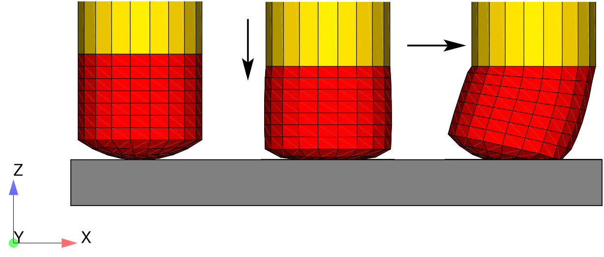
Fig. 13.3 Eraser schematic; Block 1 (yellow) is pencil, block 2 (red) is eraser, block 3 (gray) is tablet, block 4 (not shown) is tied to eraser and has the kinematics applied to it.
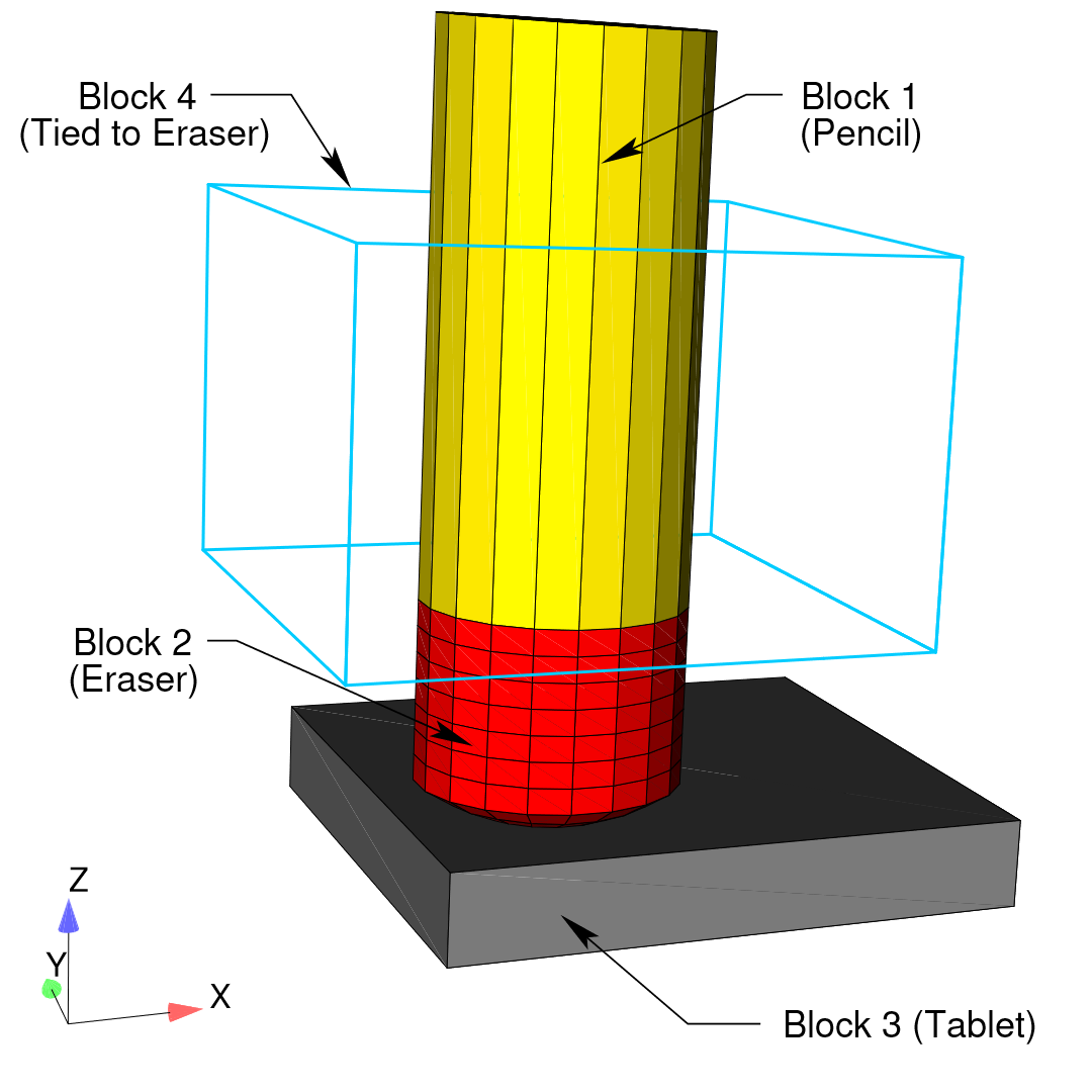
Fig. 13.4 Complete eraser mesh.
The problem kinematics and loading are described briefly here. The loading has two phases: preload and sliding. In the preload phase, the tablet (block 3) is kinematically fixed in the \(x\)-\(y\) plane and a vertical load (in the \(z\)-direction) is applied to the tablet which presses the tablet against the eraser (block 2). The eraser is kinematically fixed to block 4 via tied contact (see Fig. 13.4). Block 4 is held fixed in all three coordinate directions for the compression phase. The initial configuration and deformations of the preload phase are shown in the first two snapshots on the left in Fig. 13.3. In the sliding phase, block 4 is kinematically prescribed to move along the \(x\)-direction, thus sliding or dragging the eraser along the tablet (see Fig. 13.3) while the tablet force is held constant.
The input file is described below, with comments to explain every few lines. Following the description, the full input file is listed again. All character strings in the input file are presented in lowercase, which is an acceptable format in Adagio.
The input file starts with a begin sierra statement, as is required for all input files:
begin sierra eraser
We begin by defining vectors corresponding to the coordinate axes. These vectors/directions will be used to define the input for boundary condition blocks that come later.
define direction X with vector 1.0 0.0 0.0
define direction Y with vector 0.0 1.0 0.0
define direction Z with vector 0.0 0.0 1.0
We now need to define the functions used for this problem. The boundary conditions require a function for the tablet force and the sliding motion. Both the tablet force and sliding motion are prescribed as functions of time.
begin function slide
  type is piecewise linear
  begin values
    0.0      0.0
    1.0      0.0
    2.0      1.0
    3.0      1.0
  end values
end function slide

begin function tablet_force
  type is piecewise linear
  begin values
    0.0      0.0
    1.0      1.0
    3.0      1.0
  end values
end function tablet_force

begin function zero
  type is constant
  begin values
    0.0
  end values
end function zero
The tablet force ramps up over the time interval (0.0, 1.0) and then is held constant over the interval (1.0, 3.0). The sliding function is zero over the time interval (0.0, 1.0) and then it linearly increases over the interval (1.0, 2.0). Next, we define the material properties and models that are used in this problem. In this example, we define two sets of material properties: one is called stiff (pencil, tablet, and block 4), and the second is called soft (eraser). We use a linear elastic constitutive model for both cases.
begin material stiff
  density = 1.0
  begin parameters for model elastic
    youngs modulus = 1.e5
    poissons ratio = 0.3
  end parameters for model elastic
end material stiff

begin material soft
  density = 1.0
  begin parameters for model elastic
    youngs modulus = 1000.
    poissons ratio = 0.3
  end parameters for model elastic
end material soft
Now, we define the finite element mesh. This includes specification of the file that contains the mesh, a list of all the element blocks we will use from the mesh and the material associated with each block. The name of the file is eraser.g. The specification of the database type is optional-ExodusII is the default. Currently, each element block must be defined individually. The tablet, pencil and block 4 all reference the same material description (stiff). The material description is not repeated three times. The material description for stiff appears once and is then referenced three times.
begin finite element model mesh1
  database name = eraser.g
  database type = exodusII
  begin parameters for block block_1 #Pencil
    material = stiff
    model = elastic
  end
  begin parameters for block block_2 #Eraser
    material = soft
    model = elastic
  end
  begin parameters for block block_3 #Tablet
    material = stiff
    model = elastic
  end
  begin parameters for block block_4 #dummy block
    material = stiff
    model = elastic
  end
end finite element model mesh1
At this point we have finished specifying physics-independent quantities. We now want to set up the Adagio procedure and region, along with the time control command block. We start by defining the beginning of the procedure scope, the time control command block, and the beginning of the region scope. Three time stepping command blocks are used in this analysis. The termination time is set to 1.8. Having multiple time blocks is useful because we can make some solver options a function of the time block.
begin adagio procedure agio_procedure
  begin time control
    begin time stepping block preload
      start time = 0.0
      begin parameters for adagio region adagio
        number of time steps = 5
      end parameters for adagio region adagio
    end time stepping block preload
    begin time stepping block slide_1
      start time = 1.0
      begin parameters for adagio region adagio
        number of time steps = 1
      end parameters for adagio region adagio
    end time stepping block slide_1
    begin time stepping block slide_2
      start time = 1.1
      begin parameters for adagio region adagio
        number of time steps = 10
      end parameters for adagio region adagio
    end time stepping block slide_2
    termination time = 1.8
  end time control

  begin adagio region adagio
Next we associate the finite element model we defined above (mesh1) with this Adagio region.
use finite element model mesh1
Now we define the kinematic boundary conditions. First, we prescribe the displacement of surface_200 which is part of block 4. We fix this surface in both the \(x\) and \(z\) directions and prescribe the horizontal displacement along the X-direction using the previously defined functions zero and slide.
### movement of pencil prescribed by block 4
begin prescribed displacement
  surface = surface_200
  direction = X
  function = slide
  scale factor = 3.0
end prescribed displacement
begin fixed displacement
  surface = surface_200
  components = Y Z
end fixed displacement
Next, we fix the tablet and prevent it from moving in the X-Y plane. We do this on all tablet nodes (nodelist_111 and nodelist_112).
### Constraints on tablet
begin fixed displacement
  node set = nodelist_111
  components = X Y
end fixed displacement
begin fixed displacement
  node set = nodelist_112
  components = X Y
end fixed displacement
Finally, we prescribe preload force on the tablet which compresses the tablet against the eraser.
### Tablet force
begin prescribed force
  node set = nodelist_111
  direction = Z
  function = tablet_force
  scale factor = 100.0
end prescribed force
We now define the contact for this problem. Here we need to define tied contact between block 4 and the eraser. In addition, we have frictional sliding contact between the tablet and the eraser.
### block 4 tied to eraser ###
begin contact definition
  #
  # define contact surfaces.
  contact surface surf_200 contains surface_200
  contact surface surf_110 contains surface_110
  contact surface surf_11  contains surface_11 # Tablet
  contact surface surf_10  contains surface_10 # Eraser
  #
  begin interaction
    surfaces = surf_200 surf_110
    friction model = tied
  end interaction

  begin interaction
    surfaces = surf_11 surf_10
    friction model = fric
  end interaction

  begin constant friction model fric
    friction coefficient = 0.8
  end

end contact definition
Now we define what variables we want in the output file and how often we want the output file to be written. The output file will be called eraser.e, and it will be an ExodusII file (the database type command is optional; it defaults to ExodusII). The variables we are requesting are the displacements, velocities, and contact diagnostics at the nodes, and stresses and strains at the elements.
begin results output output_adagio
  database name = eraser.e
  database type = exodusII
  at step 0, increment = 1
  nodal displacement as displ
  nodal velocity as vel
  nodal contact_tangential_direction as cont_tan
  nodal contact_normal_direction as cont_norm
  nodal contact_accumulated_slip_vector as cont_slip_vec
  nodal contact_status as cont_stat
  nodal contact_normal_traction_magnitude as norm_trac_mag
  nodal contact_tangential_traction_magnitude as tan_trac_mag
  nodal contact_incremental_slip_magnitude as cont_Islip_mag
  nodal contact_accumulated_slip as cont_Aslip
  nodal contact_frictional_energy_density as cont_fric_E
  nodal contact_area
  element stress as stress
  element log_strain as strain
end results output output_adagio
The final part of the input deck is the Adagio solver commands. Because we are solving an implicit problem, we must use the solver command block. Nested inside the solver block, we define the control contact block as well as the nonlinear conjugate gradient (CG) solver block.
begin solver
  begin control contact name
    target relative residual = 1e-3
    Maximum Iterations = 200
  end control contact name
  begin cg
    target relative residual = 1.e-4
    begin full tangent preconditioner
      linear solver = feti
    end full tangent preconditioner
  end cg
end solver
After defining the Adagio region and procedure blocks, we close them using the lines:
  end adagio region adagio
end adagio procedure agio_procedure
The final detail that we need to define for this file is the linear solver. In the above solver command block, we included the full tangent preconditioner block, which has a nested command line linear solver = feti. This command line refers to a linear solver called feti that must be defined outside the “Procedure” scope but within the “Sierra” scope and can come at the top of the file before the “Procedure” definition or after it as is the case here. The input feti on this line command is a user defined string that can have any useful label. The following command block defines the linear solver labeled feti. Note that the command block has the label feti at the end of the Begin line and that this label is referred to from within the above full tangent preconditioner command block. The FETI parameters are all set to reasonable values for most problems, so there is no need to set any of them, but if it were necessary to set any of them to non-default values, that would be done within the feti equation solver block.
begin feti equation solver feti
  # use default settings
end feti equation solver feti
Finally, we finish the input file and close the sierra command block:
end sierra eraser