5.1. General Material Commands

A MATERIAL command block may include command lines applicable to all the material models specified within the command block. These command lines related to density, to Biot’s coefficient, and the thermal strain behavior are discussed, respectively, in Section 5.1.1, Section 5.1.2, and Section 5.1.4. Additionally several material models share similar behavior for certain commands such as elastic constants and the beta parameter discussed in Section 5.1.5 and Section 5.1.6.

5.1.1. Density Command

DENSITY = <real>density_value

This command line specifies the density of the material. The units of the input parameter density_value are mass per unit volume.

A MATERIAL command block can contain one or more PARAMETERS FOR MODEL command blocks. The specified density_value will be used with all models described in these PARAMETERS FOR MODEL command blocks.

5.1.2. Biot’s Coefficient Command

BIOTS COEFFICIENT = <real>biots_value

This command line specifies the Biot’s coefficient of the material. Biot’s coefficient is used with the pore pressure capability (commonly called an effective stress model). See Section 7.13 for more information on pore pressure. If not given, the value defaults to 1.0 which is a common value for many rock properties. This parameter is unitless. The pore pressure capability is implemented as the following effective stress model

\[\sigma_{effective} = \sigma - \alpha P\]

where P is the pressure and \(\alpha\) is Biot’s coefficient.

A MATERIAL command block can contain one or more PARAMETERS FOR MODEL command blocks. The specified biots_value will be used with all models described in these PARAMETERS FOR MODEL command blocks.

5.1.3. General Artificial Strains

Sierra/SM allows a user to apply an artificial strain to a material. Artificial strains may be applied via the Artificial Strain commands or via the Thermal Strain commands ( Section 5.1.4). General artificial strains may be useful for fitting parts together for a preload analysis or modeling a variety of other physics that could cause material expansion or contraction (such as radiation induced expansion, material desiccation, etc.)

Artificial strains may also be defined via a boundary condition. See Section 7.16.7.

The artificial strain commands are placed in the MATERIAL command block.

ARTIFICIAL ENGINEERING STRAIN FUNCTION =
  <string>artificial_strain_function
#
# Or all three of the following
#
ARTIFICIAL ENGINEERING STRAIN X FUNCTION =
  <string>artificial_strain_x_function
ARTIFICIAL ENGINEERING STRAIN Y FUNCTION =
  <string>artificial_strain_y_function
ARTIFICIAL ENGINEERING STRAIN Z FUNCTION =
  <string>artificial_strain_z_function
#
# Or one to three of the following
#
ARTIFICIAL ENGINEERING STRAIN DIRECTION
 <string>dir_name FUNCTION = <string>funcName

The ARTIFICIAL ENGINEERING STRAIN FUNCTION defines an isotropic strain.

The X, Y, and Z functions may define anisotropic strain. Note, the X, Y, and Z directions correspond to the material coordinate system. For most solid element materials, the material coordinate system is aligned with the global X, Y, and Z axes. For orthotropic solid materials, the X, Y, and Z thermal strains are applied in the material orthotropic R, S, and T coordinate system (which may vary element to element). For two dimensional shell and membrane elements, the X and Y directions are in the plane of the shell, and Z is the through thickness direction. Z strains generally have no effect on shells. See Section 6.2.5 for a discussion of the shell \(rst\) coordinate system. For one dimensional beam or truss elements, the X direction is along the length of the beam, and the Y and Z lie in the orthogonal directions. Y and Z strains generally have no effect on beams or trusses.

The STRAIN DIRECTION function defines strain in an arbitrary direction (note, still in the material coordinate system). Up to three orthogonal direction functions may be used.

All the artificial strain functions define the material engineering strain with respect to time. If a material is using artificial strain, it must define either one isotropic function or all three anisotropic functions.

It is highly important to note that there is zero artificial strain applied at the reference (original) model configuration. Thus artificial strains are calculated as the difference in strain function from the current time back to the reference time (analysis start time). For clarity, it is recommended that the artificial strain function be zero at the start time of the analysis. Artificial strain is a component of Non-Material strain; consequently, it is a strain that does not produce stress from the material response. The output variable names for artificial strain can be found in Table Table 9.15, Table Table 9.18, Table Table 9.19, Table Table 9.20, or Table Table 9.22 depending on the element type it is applied to.

5.1.4. Thermal Strain Behavior

Isotropic and orthotropic thermal strains may be defined for use by material models listed in a MATERIAL command block. Section 5.1.4.1 describes the command lines that are used to define the thermal strain behavior. These command lines must be used in conjunction with other command blocks outside of a MATERIAL command block for the calculations of thermal strains to be activated. Section 5.1.4.2 explains the process for activating thermal strains.

5.1.4.1. Defining Thermal Strains

THERMAL \{LOG|ENGINEERING\} STRAIN FUNCTION =
  <string>thermal_strain_function
#
# or all three of the following
#
THERMAL \{LOG|ENGINEERING\} STRAIN X FUNCTION =
  <string>thermal_strain_x_function
THERMAL \{LOG|ENGINEERING\} STRAIN Y FUNCTION =
  <string>thermal_strain_y_function
THERMAL \{LOG|ENGINEERING\} STRAIN Z FUNCTION =
  <string>thermal_strain_z_function
#
# Or one to three of the following
#
THERMAL \{LOG|ENGINEERING\} STRAIN DIRECTION
 <string>dir_name FUNCTION = <string>funcName

A MATERIAL command block may include command lines that define thermal strain behavior. It is possible to specify either an isotropic thermal-strain field using the command line STRAIN FUNCTION or an orthotropic thermal-strain field using the command lines STRAIN X FUNCTION, STRAIN Y FUNCTION, and STRAIN Z FUNCTION. For any of these command lines, the user supplies a thermal strain function (via a FUNCTION command block), which defines the thermal strain as a function of temperature. Thermal strain is a component of Non-Material strain; consequently, it is a strain that does not produce stress from the material response. The computed thermal strain is then subtracted from the strain passed to the material model.

Thermal strains may be specified in either engineering or log strain values. Note, the older version of these commands THERMAL STRAIN FUNCTION = specified log strain. Thermal strain data is often provided in engineering strain units, though the native strain measure inside of Adagio/Presto is log strain. At small strain values, log strain and engineering strain are nearly identical.

The THERMAL STRAIN FUNCTION defines an isotropic strain.

The X, Y, and Z functions define anisotropic strain. Note, the X, Y, and Z directions correspond to the material coordinate system. For most solid element materials, the material coordinate system is aligned with the global X, Y, and Z axes. For orthotropic solid materials, the X, Y, and Z thermal strains are applied in the material orthotropic R, S, and T coordinate system (which may vary element to element). For two dimensional shell and membrane elements, the X and Y directions are in the plane of the shell, and Z is the through thickness direction. Z strains generally have no effect on shells. See Section 6.2.5 for a discussion of the shell \(rst\) coordinate system. For one dimensional beam or truss elements, the X direction is along the length of the beam, and the Y and Z lie in the orthogonal directions. Y and Z strains generally have no effect on beams or trusses.

The STRAIN DIRECTION function defines strain in an arbitrary direction (note, still in the material coordinate system). Up to three orthogonal direction functions may be used.

If an isotropic thermal strain field is to be applied, the THERMAL {LOG|ENGINEERING} STRAIN FUNCTION command line is placed in the MATERIAL command block outside of the specifications of any material models. Such placement is necessary because the isotropic thermal strain is a general material property, not a property that is specific to any particular constitutive model such as ELASTIC or ELASTIC-PLASTIC. The input value of thermal_strain_function is the name of the function that defines thermal strain as a function of temperature for the material model described in this particular MATERIAL command block. The function is defined within the SIERRA scope using a FUNCTION command block. For more information on how to set the input to compute thermal strains and how to apply temperatures, see Section 5.1.4.2.

The specification of an orthotropic thermal strain field requires that all three of the THERMAL STRAIN X FUNCTION, THERMAL STRAIN Y FUNCTION, and THERMAL STRAIN Z FUNCTION command lines be placed in the MATERIAL command block. All three command lines must be provided, even when there is no thermal strain in one or more directions. The values of thermal_strain_x_function, thermal_strain_y_function, and thermal_strain_z_function are the names of the functions for thermal strains in the \(X\)-direction, the \(Y\)-direction, and the \(Z\)-direction, respectively. These functions are defined within the SIERRA scope using FUNCTION command blocks. To specify that there should be no thermal strain in a given direction, use a function that always evaluates to zero for that direction.

If one the THERMAL {LOG|ENGINEERING STRAIN FUNCTION} command lines are used for one of the several of the material models, as discussed in Section 5.1.4.2. The model external artificial strain and the model internal artificial strain will be multiplied together. The use of a thermal strain is identified in the descriptions of the material models in Section 5.2 by the notation thermal strain option.

If both artificial and thermal strain are defined simultaneously the two strain components are additive.

The output variable names for thermal strain can be found in Table Table 9.13.

5.1.4.2. Activating Thermal Strains

Sierra/SM has the capability to compute thermal strains on three-dimensional continuum, two-dimensional (shell, membrane), and one-dimensional (beam, truss) elements. Three inputs are required to activate thermal strains:

One or more thermal strain functions (strain as a function of temperature) must be defined. Each thermal strain function is defined with a FUNCTION command block. (This function is the standard function definition that appears in the SIERRA scope.) The thermal strain function gives the total thermal strain associated with a given temperature. It is the change in thermal strain with the change in temperature that gives rise to thermal stresses in a body.
The material models used by blocks that experience thermal strain must have their thermal strain behavior defined. The command lines for defining isotropic and orthotropic thermal strain are described in Section 5.1.4.1. Materials with isotropic thermal strain use the THERMAL {LOG|ENGINEERING} STRAIN FUNCTION command line, while those with orthotropic thermal strain must define thermal strain in all three directions using the THERMAL {LOG|ENGINEERING} STRAIN X FUNCTION, THERMAL {LOG|ENGINEERING} STRAIN Y FUNCTION, and THERMAL {LOG|ENGINEERING} STRAIN Z FUNCTION command lines. These inputs can be used with all material models with the exception of the following: elastic three-dimensional orthotropic, Mooney-Rivlin, NLVE three-dimensional orthotropic, Swanson, and viscoelastic Swanson. These models require their own model-specific inputs to define thermal strain and must not use these standard commands. Information for defining thermal strains is provided in the individual descriptions of these models in Section 5.2.
A temperature field must be applied to the affected blocks. The boundary condition command block to specify the application of temperatures is PRESCRIBED TEMPERATURE. A description of the PRESCRIBED TEMPERATURE command block is given in Section 7.12.

An applied temperature is prescribed at the nodes, but thermal strain is computed based on element temperature. Element temperatures are obtained by averaging the temperatures of the nodes connected to a given element.

It is important to note that there is zero thermal strain applied at the reference temperature. The thermal strain reference temperature is stored in the element field named “thermal_strain_reference_temperature” and may vary from element to element. Unless otherwise specified, the thermal strain reference temperature for each element is given by the initial temperature for that element, i.e., the model without other loads is in a stress-free state at the initial temperature. If desired, a different stress-free reference temperature can be used by prescribing the reference temperature with the INITIAL CONDITION command block as described in Section 7.3.

A second critical note is that thermal strain is applied based the change in temperature over a step. First the temperature is computed at the beginning of the step and the end of the step. Next the thermal strain is computed at these beginning and end of the step temperatures. The thermal strain increment is computed by the difference of these beginning and end of step strains. Finally this strain increment is applied to the material. Due to this thermal strain enforcement process the thermal strain is affected only by the slope of the thermal strain function. A vertical offset of the thermal strain function has no effect. Additionally if two discontinuous temperature functions are applied in different time periods thermal strain will not see the temperature jump between these two functions.

5.1.4.3. Thermal Strain Example

Example Consider the following thermal strain function:

BEGIN FUNCTION thermStrain
  TYPE IS PIECEWISE LINEAR
  BEGIN VALUES
    500  -0.04
    1000  0.01
    1500  0.03
  END
END

Let an element have an initial temperature of 1000 and a thermal strain reference temperature of 1000. Initially the element has zero applied thermal strain as it is at the strain-free reference temperature. If the element heats to temperature 1500, the thermal strain applied to the element will be 0.02 (the thermal strain at 1500 minus the thermal strain at the reference temperature 1000). If the element cools to 500, the thermal strain applied to the element will be -0.05 (the thermal strain at 500 minus the thermal strain at the reference temperature 1000).

5.1.5. Elastic Constants

YOUNGS MODULUS = <real>
POISSONS RATIO = <real>
SHEAR MODULUS  = <real>
BULK MODULUS   = <real>
LAMBDA         = <real>
TWO MU         = <real>

Many material models contain input for basic elastic constants. These elastic constants may define the material response before yield, the elastic unloading response, or the approximate elastic stiffness of the material model. There exist several inter-related ways to define the elastic material properties. Six separate elastic constants may potentially be set YOUNGS MODULUS (\(E\)), POISSONS RATIO (\(\nu\)), BULK MODULUS (\(K\)), SHEAR MODULUS (\(G\)), LAMBDA (\(\lambda\)), and TWO MU (\(2\mu\)).

Generally elastic constants may either be set within the BEGIN MATERIAL command block or the BEGIN PARAMETERS FOR MODEL .... command block. Constants defined in the BEGIN MATERIAL block apply to all models in the material block. Constants defined in the BEGIN PARAMETERS FOR MODEL .... block apply to just that specific material model.

The parsed elastic constants are echoed to the log file when reading the material to verify correct setup. For example:

MATERIAL ELASTIC CONSTANT:steel_ELASTIC

E           Nu          G           K           Lambda
7.43e+11    0.34        2.77e+11    7.74e+11    5.89e+11

Note, the elastic constants printed at this point in the log are based off of the raw values of the global elastic constants such as YOUNGS MODULUS. The printed constants are not scaled for temperature dependence or any other external scaling factors. The proper element-by-element scaling will ultimately be used by the element mechanics and can be viewed by plotting the element variables dilmod (Dilatational Modulus) and shrmod (Shear Modulus.)

Examples:

#
#  Define elastic constants for a specific material model
#
BEGIN MATERIAL steel
  BEGIN PARAMETERS FOR MODEL ELASTIC
    YOUNGS MODULUS = 200e+9
    POISSONS RATIO = 0.3
  END
END

#
#  Define elastic constants for all associated material models
#
BEGIN MATERIAL aluminum
  YOUNGS MODULUS = 40e+9
  POISSONS RATIO = 0.35

  BEGIN PARAMETERS FOR MODEL ELASTIC
    ....
  END
  BEGIN PARAMETERS FOR MODEL ELASTIC_PLASTIC
    ....
  END
END

The elastic properties are defined as follows:

YOUNGS MODULUS describes the tensile elasticity, how much an object strains when it is pulled with opposing forces. Young’s modulus must be a non-negative number.
POISSONS RATIO describes how much a material expands laterally in unconstrained compression. An incompressible material has a Poisson’s ratio of 0.5. The valid range for Poisson’s ratio if from {-1} to {0.5}.
BULK MODULUS describes the volumetric elasticity, how much an object shrinks under isotropic compression. Bulk modulus must be a non-negative number.
SHEAR MODULUS describes the resistance of a solid to shear forces. A freely flowing fluid would have zero shear modulus. Shear modulus must be a non-negative number.
LAMBDA is the first Lame elastic constant. Lambda can have any value though is generally positive for real materials.
TWO MU is twice the shear modulus.

The elastic constants are interrelated and defining any two of these constants (with the exception of TWO MU and SHEAR MODULUS) fully defines the elastic properties of the material. Generally exactly two of these constants should be set for each material model. Note, TWO MU and SHEAR MODULUS define the same constant (TWO MU is just twice the SHEAR MODULUS). Thus TWO MU and SHEAR MODULUS should not be defined at the same time.

Given Young’s Modulus \(E\) and Poisson’s ratio (\(\nu\)) the other four elastic constants would be set as follows:

\[\begin{split}\texttt{BULK MODULUS}: \;\;\; & K = \frac{E}{3(1 - 2 \nu)} \\ \texttt{SHEAR MODULUS}: \;\;\; & G = \frac{E}{2( 1 + \nu)} \\ \texttt{LAMBDA}: \;\;\; & \lambda = \frac{E \nu}{(1 + {\nu})(1 - 2 \nu )} \\ \texttt{TWO MU}: \;\;\; & 2\mu = \frac{E}{1 + \nu}\end{split}\]

5.1.6. The Isotropic/Kinematic hardening BETA parameter

BETA = <real>betaVal(1.0)

Several plasticity model variants make use of the Isotropic/Kinematic hardening factor BETA. In a three-dimensional framework, hardening is the law that governs how the yield surface evolves in stress space. If the yield surface grows uniformly in stress space, the hardening is called isotropic hardening. When BETA is 1.0 the model uses only isotropic hardening. If the yield surface does not grow in stress space but rather moves, the hardening is called kinematic hardening. When BETA is 0.0 the model uses only kinematic hardening. Values of BETA between 0.0 and 1.0 define a mixture of isotropic and kinematic hardening. Note, the input BETA has other meanings in some models, so see the specific material model documentation for details.

The mechanics of isotropic hardening are demonstrated in Fig. 5.1.

../../_images/isotropic_hard.png — Fig. 5.1 Isotropic hardening, `BETA = 1.0`.

The mechanics of kinematic hardening are demonstrated in Fig. 5.2. If using pure kinematic hardening, then irrespective of the post yield hardening behavior the yield surface will never grow larger than the initial yield stress. Thus when using pure kinematic hardening the particular shape of the post yield hardening curve generally has no effect.

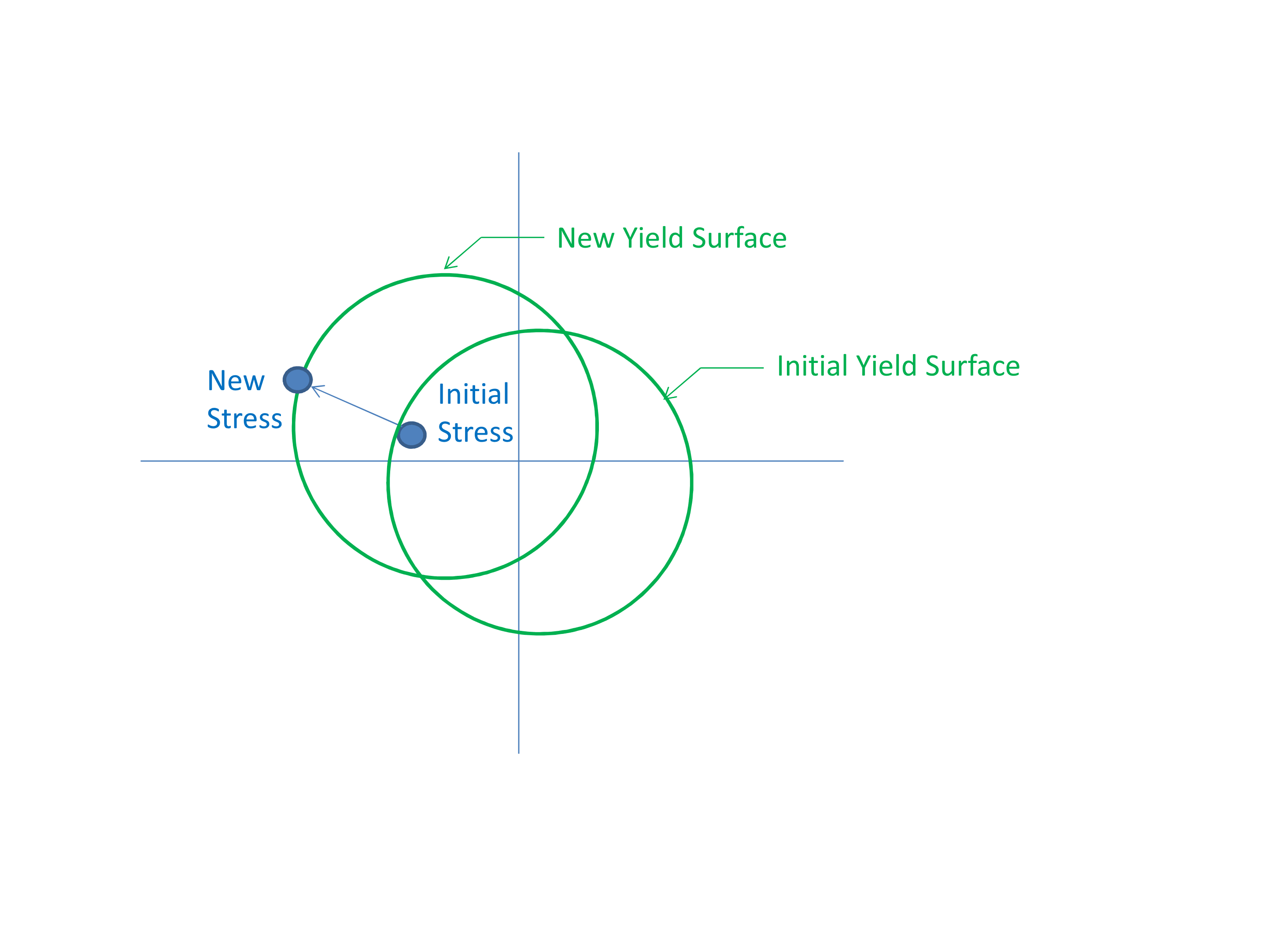
../../_images/kinematic_hard.png — Fig. 5.2 Kinematic hardening, `BETA = 0.0`.

The mechanics of a mixed 0.5 BETA parameter is demonstrated in Fig. 5.3.

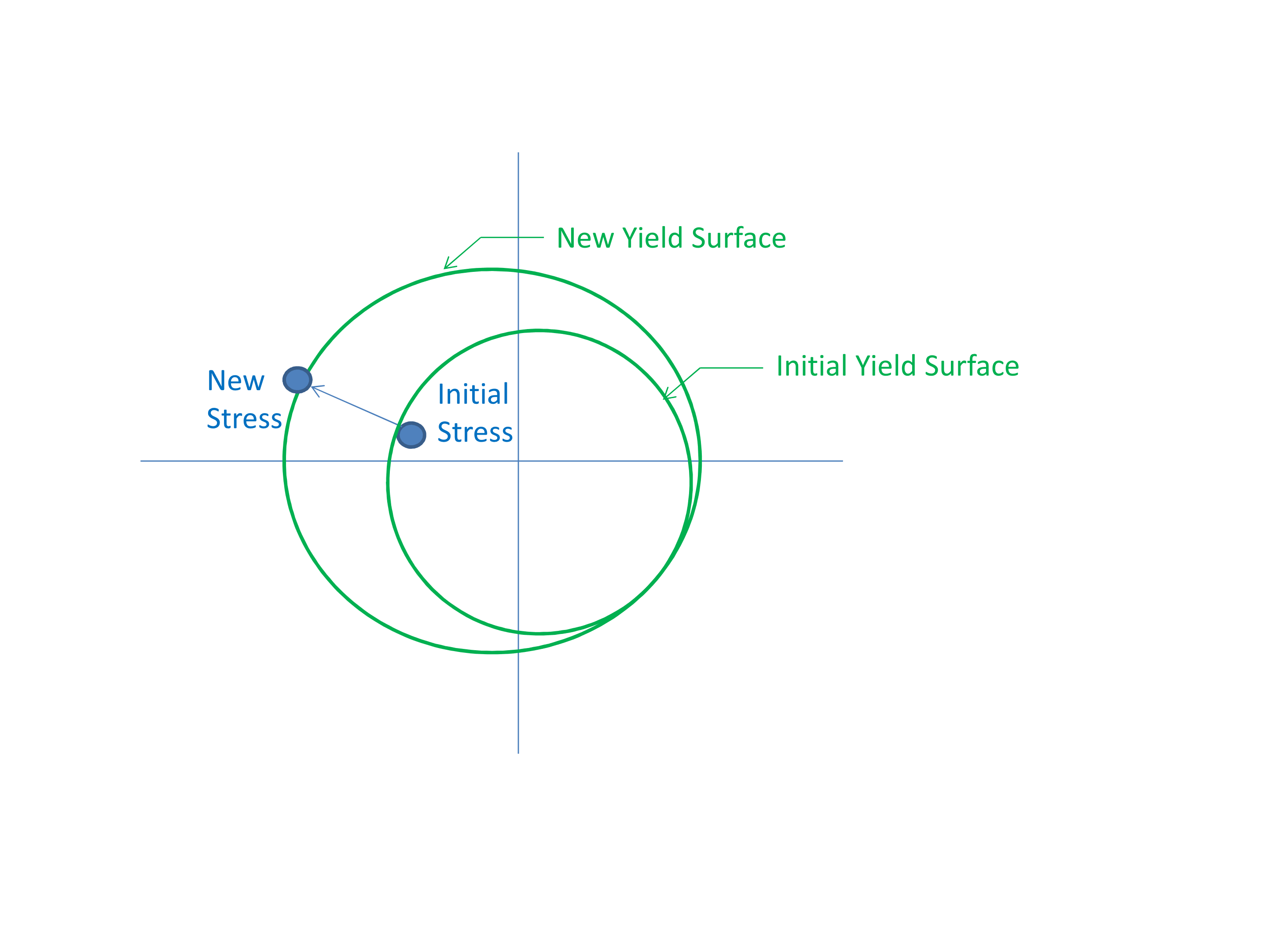
../../_images/mixed_hard.png — Fig. 5.3 Mixed hardening, `BETA = 0.5`.

5.1.7. Coordinate Systems

COORDINATE SYSTEM             = <string> coordinate_system_name
DIRECTION FOR ROTATION        = <real> 1|2|3
ALPHA                         = <real> (degrees)
SECOND DIRECTION FOR ROTATION = <real> 1|2|3
SECOND ALPHA                  = <real> (degrees)

Several anisotropic materials can be tied to an element specific coordinate frame. By default the material R, S, and T coordinate frame lines up with the global X, Y, and Z coordinate system. A different material R, S, and T coordinate frame can be defined with the above commands, for example to define material properties that vary in the hoop and radial directions of a cylinder.

Note, in addition to the coordinate system commands listed here, some material models have other model specific coordinate system options.

The specification of the principal material directions begins with the selection of a user-specified coordinate system given by the COORDINATE SYSTEM command line. The coordinate_system_name references a coordinate system defined by a separate COORDINATE SYSTEM command blocks (see Section 2.1.9). COORDINATE SYSTEM defines a local R, S, and T frame for each element based on the element centroid. This initial coordinate system can then be rotated twice to give the final material directions at each material point.

The first rotation of the initial coordinate system is defined using the DIRECTION FOR ROTATION and ALPHA command lines. The axis for rotation of the initial coordinate system is specified by the DIRECTION FOR ROTATION command line, 1 corresponds to the initial coordinate system local R axis, 2 corresponds to the initial coordinate system local S axis, and 3 corresponds to the initial coordinate system local T axis. The right hand rule angle of rotation about this axis is given by ALPHA. This rotation yields an intermediate coordinate system.

A secondary rotation of the intermediate coordinate system may be defined using the SECOND DIRECTION FOR ROTATION and SECOND ALPHA command lines. The axis for rotation of the intermediate coordinate system is specified by the SECOND DIRECTION FOR ROTATION command line, 1 corresponds to the intermediate coordinate system local R axis, 2 corresponds to the intermediate coordinate system local S axis, and 3 corresponds to the intermediate coordinate system local T axis. The right hand rule angle of rotation about this axis is given by SECOND ALPHA. The resulting coordinate system gives the final R, S, and T coordinate frame for the material directions.