4.25. Shape Memory Alloy Model

4.25.1. Theory

The shape memory alloy (SMA) model is used to describe the thermomechanical response of intermetallics (e.g. NiTi, NiTiCu, NiTiPd, NiTiPt) that can undergo a reversible, diffusionless, solid-to-solid martensitic transformation. Specifically, the materials have a high-symmetry (typically cubic) austenitic crystallographic structure at high temperature and/or low stress. At lower-temperatures and/or high stress the crystallographic structure is transformed to a lower symmetry (typically orthorhombic or monoclinic) martensitic phase. The change in structure and symmetry may be taken advantage of to produce large inelastic strains of \(\approx\) 1-8%. Importantly, this class of materials differentiates itself from TRIP steels in that the transformation is reversible and a variety of thermomechanical loading paths have been conceived of to take advantage of this behavior. A notable application of these materials is as an actuator in smart, morphing structures.

Phenomenologically, the macroscopic behavior of SMAs is typically discussed in effective stress-temperature space via a phase diagram like in Fig. 4.117. The four lines denoted \(M_s,~M_f,~A_s,\) and \(A_f\) indicate the martensitic start, martensitic finish, austenitic start, and austenitic finish transformation surfaces. Forward transformation (from an austenitic to a martensitic state) is described by the martensitic start and finish surfaces. Specifically, the former refers to the thermomechanical conditions at which transformation will initiate while the latter corresponds to complete transformation. The difference between the two surfaces is associated with internal hardening effects due to microstructure (i.e. texture, back stresses). Transformation from martensite to austenite is referred to as reverse and is characterized by the austenitic start and finish surfaces. Detailed discussion of the crystallography and phenomenology may be found in [[1], [2]] (In the martensitic configuration, the crystallographic structure can either self-accommodate in a twinned configuration producing no macroscopic inelastic strain or an internal or external stress field may be used to detwin the microstructure thereby producing the desired inelastic strain. For simplicity, this distinction is bypassed in this brief text and the interested reader should consult the referenced works.).

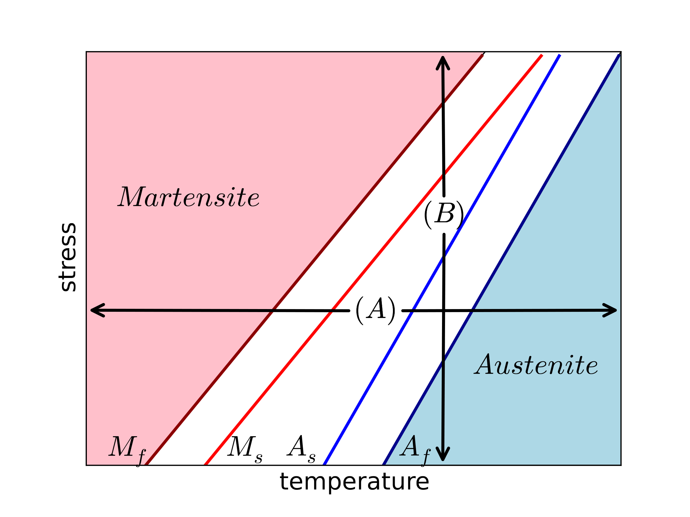
Fig. 4.117 Representative phase diagram of shape memory alloys highlighting characteristic loading paths (\(\left(A\right)\) and \(\left(B\right)\)), transformation surfaces, and phases.

Two responses characteristic of SMAs may also be represented via the phase diagram. These are the actuation response and the pseudoelastic (often referred to as superelastic in the literature) responses. The first (actuation) is indicated by path \(A\) in Fig. 4.117. In this case, a mechanical bias load is applied to the SMA and the material is then thermally cycled through forward and reverse transformation. The resulting transformation first produces and then removes the large transformation strains of SMAs and is commonly used for (surprisingly) actuation applications. At higher temperatures (\(T>A_f\)), mechanical loading may be used induce forward and, upon unloading, reverse transformation as indicated in path \(B\) of Fig. 4.117. Through such a cycle, a distinctive flag shape in the stress strain response is observed through which large amounts of energy may be dissipated while producing no permanent deformations. As such, this loading path is often considered for vibration isolation or damping applications.

In LAME, the response of SMAs is described by the phenomenological model of Lagoudas and coworkers [[3]]. This model was motivated by actuator applications and it describes the inelastic deformation associated with martensitic transformation through two internal state variables – the scalar martensitic volume fraction, \(\xi\), and tensorial transformation strain tensor, \(\varepsilon^{\text{tr}}_{ij}\). Before proceeding it should be noted that the structural response of SMA specimens and components exhibit a rate dependency associated with the strong thermomechanical coupling of SMAs. Specifically, the transformation process gives off/absorbs large amounts of energy via the latent heat of transformation. The rate dependence observed is a result of the characteristic time scale associated with thermal transport of this heat. In pure mechanical analyses (like Sierra/SM), this means quasistatics loadings are typically considered (a strain rate of \(\approx 1x10^{-4}\) and/or heating/cooling rate of \(\approx 2^{\circ}C/\text{min}\)). Formulations accounting for the full coupling have been developed but require more complex implementations.

To begin, the model assumes an additive decomposition of the total, elastic, thermal, and transformation deformation (strain) rates respectively denoted by \(D_{ij},~D^{\text{e}}_{ij},~D^{\text{th}}_{ij}\) and \(D^{\text{tr}}_{ij}\) producing a total deformation rate of the form,

\[D_{ij}=D^{\text{e}}_{ij}+D^{\text{th}}_{ij}+D^{\text{tr}}_{ij}.\]

With respect to the thermoelastic deformations, it is noted that the different crystallographic phases have different thermoelastic constants. Previous studies have demonstrated that a rule of mixtures on the compliance and other material properties of the form,

\[\begin{split}\mathbb{S}_{ijkl}=\mathbb{S}_{ijkl}^A+\xi\left(\mathbb{S}_{ijkl}^M-\mathbb{S}_{ijkl}^A\right)=\mathbb{S}_{ijkl}^A+\xi\Delta \mathbb{S}_{ijkl}, \\ \mathbb{\alpha}_{ij}=\alpha^A\delta_{ij}+\xi\left(\alpha^M\delta_{ij}-\alpha^A\delta_{ij}\right)=\alpha^A\delta_{ij}+\xi\Delta\alpha\delta_{ij},\end{split}\]

in which \(\mathbb{S}_{ijkl}\) and \(\alpha_{ij}\) are the current effective compliance and coefficient of thermal expansion and the superscripts \(A\) and \(M\) denote thermoelastic properties in the austenitic and martensitic configuration. The symbol \(\Delta\) is used to indicate the difference in a property between the martensitic and austenitic phases while \(\delta_{ij}\) is the Kronecker delta. Isotropy is assumed for all these properties and the compliances are determined via the definition of elastic moduli and Poisson’s ratio of the two phases – \(E^A\), \(E^M\), \(\nu^M\), and \(\nu^M\). The two Poisson ratios are often the same and take typical values for metals (\(\nu^A\approx\nu^M\approx 0.3\)) while the elastic moduli can differ by a factor of more than two. For instance the austenitic modulus of NiTi is typically given as \(\approx\) 70 GPa while the martensitic one is \(\approx\) 30 GPa (Given the lower symmetry of the martensitic phase the determination of an isotropic elastic modulus can vary with characterization methodology. In this case, the apparent elastic modulus measured from macroscopic thermoelastic tests should be used.). Importantly, this difference means that the thermoelastic properties and corresponding deformations vary with transformation. As such, the corresponding rates of deformation are given as,

\[\begin{split}D^{\text{e}}_{ij}=\dot{\xi}\Delta \mathbb{S}_{ijkl}\sigma_{kl}+\mathbb{S}_{ijkl}\stackrel{\circ}{\sigma}_{kl}, \\ D^{\text{th}}_{ij}=\dot{\xi}\Delta\alpha\delta_{ij}\left(\theta-\theta_0\right)+\alpha\delta_{ij}\dot{\theta},\end{split}\]

where \(\theta\) and \(\theta_0\) are the current and reference temperature and \(\sigma_{ij}\) is the symmetric Cauchy stress. Note, in using the SMA model a temperature field must be defined. The stress rate may then be shown to be,

\[\stackrel{\circ}{\sigma}_{ij}=\mathbb{C}_{ijkl}\left(D_{kl}-\alpha\delta_{kl}\dot{\theta} -\dot{\xi}\left(\Delta\mathbb{S}_{klmn}\sigma_{mn}+\Delta\alpha\delta_{kl}\left(\theta-\theta_0\right)\right) -D^{\text{tr}}_{kl}\right),\]

with \(\mathbb{C}_{ijkl}\) being the current stiffness tensor defined as \(\mathbb{C}_{ijkl}=\mathbb{S}^{-1}_{ijkl}\).

To describe the transformation strain evolution, it is assumed that these deformations evolve with (and only with) the martensitic volume fraction, \(\xi\). The corresponding flow rule is given as,

\[D_{ij}^{\text{tr}}=\dot{\xi}\Lambda_{ij},\]

and \(\Lambda_{ij}\) is the transformation direction tensor assumed to be of the form,

(4.116)\[\begin{split}\Lambda_{ij}=\left\{\begin{array}{cc}H^{\text{cur}}\left(\bar{\sigma}_{vM}\right)\frac{3}{2}\frac{s_{ij}}{\bar{\sigma}_{vM}} & \dot{\xi}\geq 0 \\ \frac{\varepsilon^{\text{tr}-rev}_{ij}}{\xi^{rev}} & \dot{\xi} < 0 \end{array} \right. .\end{split}\]

In (4.116), \(H^{\text{cur}}\) is the transformation strain magnitude that is dependent on the von Mises effective stress, \(\bar{\sigma}_{vM}\), and \(s_{ij}\) is the deviatoric stress. With forward transformation defined in this way, it is assumed that deformation is shear-based and follows a \(J_2\) like flow direction. For reverse transformation (\(\dot{\xi}<0\)), the postulated form is utilized to ensure complete recovery of transformation strains with martensitic volume fraction. In other words, all transformation strain components are zero-valued at \(\xi=0\). Without enforcing this condition in this way, non-proportional loading paths could be constructed producing a non-zero transformation strain when the material is austenitic. The transformation strain at load reversal, \(\varepsilon^{\text{tr}-rev}_{ij}\), and martensitic volume fraction at load reversal, \(\xi^{rev}\), are then tracked (via the implementation) and used for this purpose.

The transformation strain magnitude, \(H^{\text{cur}}\), is a function of the von Mises effective stress (\(\bar{\sigma}_{vM}\)) and is introduced to incorporate detwinning effects without introducing an additional internal state variable complicating the model. Specifically, at low stress values, this function returns a minimum value. If the microstructure is self-accommodated this value will be zero. A decaying exponential is used such that as the stress increases the value of the strain magnitude becomes that of the maximum value incorporating both crystallographic and texture effects. The given functional form is,

\[\begin{split}H^{\text{cur}}=\left\{\begin{array}{cc} H_{\text{min}} & \bar{\sigma}_{vM} \leq \sigma_{\text{crit}} \\ H_{\text{min}} + \left(H_{\text{sat}}-H_{\text{min}}\right)\left(1-\exp\left(-k\left(\bar{\sigma}_{vM} -\sigma_{\text{crit}}\right)\right)\right) & \bar{\sigma}_{vM} > \sigma_{\text{crit}} \end{array} \right. ,\end{split}\]

where \(H_{\text{min}},~H_{\text{sat}},~k,\) and \(\sigma_{\text{crit}}\) are model parameters giving the minimum transformation strain magnitude, maximum transformation strain magnitude, exponential fitting parameter governing the transition zone, and critical stress values (in some ways analogous to the detwinning stress).

The evolution of martensitic transformation process is governed by a transformation function serving an analogous role to the yield function in plasticity. This function is given by,

\[f\left(\sigma_{ij},\theta,\xi\right)=\pm\phi\left(\sigma_{ij},\theta,\xi\right)-\bar{\sigma}\left(\sigma_{ij}\right),\]

with \(\phi\) begin the thermodynamic driving force for transformation and \(\bar{\sigma}\) the critical value. The \(\pm\) is used to denote either forward (\(+\)) or reverse (\(-\)) transformation. This transformation function and the associated forms are derived from continuum thermodynamic considerations and the details of that process are neglected here for brevity but may be found in [[3]]. The functional forms of these variables are given as,

\[\begin{split}\phi\left(\sigma_{ij},\theta,\xi\right) & = \sigma_{ij}\Lambda_{ij}+\frac{1}{2}\sigma_{ij}\Delta\mathbb{S}_{ijkl}\sigma_{kl}+\sigma_{ij}\Delta\alpha\delta_{ij}\left(\theta- \theta_0\right)+\rho\Delta s_0\theta-\rho\Delta u_0-f^t\left(\xi\right),\nonumber \\ \bar{\sigma}\left(\sigma_{ij}\right) & = \sigma_0+D\sigma_{ij}\Lambda_{ij},\end{split}\]

in which \(\rho\Delta s_0\) and \(\rho\Delta u_0\) are the differences in reference entropy and internal energy of the two phases, \(D\) is a calibration parameter intended to capture variations in dissipation with stress, and \(f^t\left(\xi\right)\) is the hardening function. With respect to this latter term, empirical observations were used to arrive at a postulated form of,

\[\begin{split}f^t\left(\xi\right)=\left\{\begin{array}{cc}\frac{1}{2}a_1\left(1+\xi^{n_1}-\left(1-\xi\right)^{n_2}\right)+a_3 & \dot{\xi}\geq 0 \\ \frac{1}{2}a_2\left(1+\xi^{n_3}-\left(1-\xi\right)^{n_4}\right)-a_3 & \dot{\xi}<0\end{array}\right. ,\end{split}\]

with \(a_1,~a_2,\) and \(a_3\) being fitting parameters and \(n_1,~n_2,~n_3,\) and \(n_4\) are exponents fit to match the smooth transformation from elastic to inelastic deformations at the start of forward, end of forward, start of reverse, and end of reverse transformation respectively.

Before proceeding, one final note should be given in regards to calibration. Specifically, some of the model parameters just listed (\(a_1,~a_2,~a_3,~D,~\sigma_0,~\rho\Delta s_0\) and \(\rho\Delta u_0\)) are not easily identified or conceptualized in terms of common thermomechanical experiments. Some easily identifiable parameters (\(M_s,~M_f,~A_s\), and \(A_f\)), however, are not evident in the theoretical formulation. Conditions associated with these terms and some physical constraints may be used to determine the model parameters in terms of these more accessible properties. These relations are,

(4.117)\[\begin{split}\rho\Delta s_0=\frac{-2\left(C^MC^A\right)\left[H^{\text{cur}}\left(\sigma\right)+\sigma\frac{\partial H^{\text{cur}}}{\partial\sigma} +\sigma\left(\frac{1}{E^M}-\frac{1}{E^A}\right)\right]}{C^M+C^A}|_{\sigma=\sigma^*}, \\ D = \frac{\left(C^M-C^A\right)\left[H^{\text{cur}}\left(\sigma\right)+\sigma\frac{\partial H^{\text{cur}}}{\partial\sigma} +\sigma\left(\frac{1}{E^M}-\frac{1}{E^A}\right)\right]}{\left(C^M+C^A\right)\left[H^{\text{cur}}\left(\sigma\right) + \sigma\frac{\partial H^{\text{cur}}}{\partial\sigma}\right]}|_{\sigma=\sigma^*}, \\ a_1=\rho\Delta s_0\left(M_f-M_s\right),~\qquad~a_2=\rho\Delta s_0\left(A_s-A_f\right), \\ a_3=-\frac{a_1}{4}\left(1+\frac{1}{n_1+1}-\frac{1}{n_2+1}\right)+\frac{a_2}{4}\left(1+\frac{1}{n_3+1}-\frac{1}{n_4+1}\right), \\ \rho\Delta u_0=\frac{\rho\Delta s_0}{2}\left(M_s+A_{f}\right),~\qquad~\sigma_0=\frac{\rho\Delta s_0}{2}\left(M_s-A_f\right)-a_3,\end{split}\]

in which \(\sigma^*\) is the scalar stress measure in which the calibration is performed at. For additional discussion on the characterization of SMAs and calibration of this model, the user is referred to [[4], [5]].

4.25.2. Implementation

Similar to the various plasticity models in LAMÉ, an elastic predictor-inelastic corrector approach is used to perform the stress updating routine. Unlike the other models, however, in the shape memory alloy routine a convex cutting plane (CCP) return mapping algorithm (RMA) is used in lieu of the closest point projection. This difference essentially simplifies the integration of flow rule and the corresponding problem at the cost of some algorithmic stability. Prior studies [[6]] have shown that this implementation is sufficient for convergence in most cases while providing a substantial savings in cost. The specific implementation used here is that of [[3]].

To compute an elastic trial state, a trial stress is determined assuming purely thermoelastic deformations such that,

\[T^{tr}_{ij} = \mathbb{C}_{ijkl}\left(\xi^n\right)\left(d_{kl}\Delta t - \alpha_{kl}\left(\xi^n\right)\Delta \theta\right), ~\qquad~ \Delta \theta = \theta^{n+1}-\theta^n.\]

In this case, it is assumed that the temperature fields are known at \(t_{n+1}\) and \(t_n\) (denoted \(\theta^{n+1}\) and \(\theta^n\), respectively) and the thermoelastic properties are computed using the martensitic volume fraction at the previous time step \(\xi^n\). At this stage, a perturbation stress (\(T_{ij}^{per}=T_{ij}^n+\beta\left(T^{tr}_{ij}-T^n_{ij}\right)\) with \(\beta<<1\)) is computed and used to determine local variations of the thermodynamic driving force, \(\phi\). This is necessary to determine the direction of transformation (forward or reverse). Using the full trial stress to this end can produce spurious results in some thermally-driven cases. The trial yield function value is then computed as,

\[f^{tr}=f\left(T_{ij}^{tr},\theta^{n+1},\xi^n\right)=\pm\phi\left(T_{ij}^{tr},\theta^{n+1},\xi^n\right)-\bar{\sigma}\left(T_{ij}^{tr}\right).\]

If \(f^{tr}<0\), no nonlinear deformation occurs and the trial solution is accepted as the material state at \(t=t_{n+1}\). When this condition is not satisfied, the CCP-RMA routine is used to correct the trial state and return it to the yield surface.

To perform the inelastic correction, the Newton-Raphson method is iteratively used to update the material state (\(T_{ij}\) and \(\xi\)) until convergence is achieved. Denoting the current and next iteration by \(\left(k\right)\) and \(\left(k+1\right)\), respectively, produces updating expressions of the form,

\[\begin{split}T_{ij}^{\left(k+1\right)} & = T_{ij}^{\left(k\right)}+\Delta T_{ij}, \nonumber \\ \xi^{\left(k+1\right)} & = \xi^{\left(k\right)}+\Delta \xi,\end{split}\]

with \(\xi^{\left(0\right)}\) and \(T_{ij}^{\left(0\right)}\) initialized to \(\xi^{n}\) and \(T_{ij}^{tr}\), respectively. The key difference between the CCP and closest point projection (CPP) methods is associated with how the inelastic strain flow rules are integrated. In the former method, an explicit evaluation of the flow direction is utilized while the latter is associated with a fully implicit expression. For the CPP algorithms, this implicit expression means the flow rule must be solved in a nonlinear system of equations with the consistency equation. Relaxing this assumption via the CCP method, however, produces an explicitly evaluated flow rule of,

\[\varepsilon^{t\left(k+1\right)}_{ij}=\varepsilon^{t\left(k\right)}_{ij}+\Delta \xi\Lambda_{ij}^{\left(k\right)}.\]

Importantly, this means that the only nonlinear equation to be solved is the scalar consistency equation (\(f=0\)) which can be linearized such that,

\[\Delta \xi = -\frac{f^{\left(k\right)}}{\frac{\partial f^{\left(k\right)}}{\partial\xi}-\frac{\partial f^{\left(k\right)}}{\partial T_{ij}} \mathbb{C}_{ijkl}\left(\xi^{\left(k\right)}\right)\left(\Delta\mathbb{S}_{klmn}T^{\left(k\right)}_{mn}+ \Delta\alpha_{kl}\Delta\theta+\Lambda^{\left(k\right)}_{kl}\right)},\]

and the stress increment is then found as,

\[\Delta T^{\left(k\right)}=-\mathbb{C}_{ijkl}\left(\xi^{\left(n\right)}\right)\left(\Delta\mathbb{S}_{klmn}T^{\left(k\right)}_{mn} + \Delta\alpha_{kl}\Delta\theta+ \Lambda^{\left(k\right)}_{kl}\right)\Delta\xi.\]

4.25.3. Verification

The shape memory alloy model is verified through a series of thermomechanical loadings. The material properties and model parameters for these investigations are given in Table 4.37. These properties correspond to those given in Table 3.4 in [[1]] with all \(n'`s assumed to be 1 and setting :math:`E^M=E^A\).

Table 4.37 The material and model parameters for the shape memory alloy model used during verification test.

\(E^A\)	55 GPa	\(E^M\)	55 GPa
\(\nu^A\)	0.33	\(\nu^M\)	0.33
\(\alpha^A\)	22.0\(x10^{-6}\frac{1}{\text{K}}\)	\(\alpha^M\)	22.0\(x10^{-6}\frac{1}{\text{K}}\)
\(M_s\)	245 K	\(A_s\)	270 K
\(M_f\)	230 K	\(A_f\)	280 K
\(C^M\)	7.4 \(\frac{\text{MPa}}{\text{K}}\)	\(C^A\)	7.4 \(\frac{\text{MPa}}{\text{K}}\)
\(H_{\text{min}}\)	0.056	\(H_{\text{sat}}\)	0.056

It should also be clear that because \(H_{\text{min}}=H_{\text{sat}}\) the model response is independent of the values of \(\sigma^{\text{crit}}\) and \(k\). For convenience, values of \(k=1.0x10^{6}\) and \(\sigma^{\text{crit}}=0\) will be used. Additionally, \(\sigma^*\) will be taken to be zero although inspection of (4.117) and consideration of the relative magnitudes of the transformation strain and the difference in elastic strain similarly indicates an invariance in the model response to this parameter with constant \(H^{\text{cur}}\). The default prestrain values are also utilized such that the SMA is initially austenitic.

4.25.3.1. Uniaxial Stress – Pseudoelasticity

First, the isothermal (\(\theta>A_f\)) pseudoelastic response through a uniaxial stress loading is explored. Importantly, the simplifications and model parameters described above (\(E^A=E^M=E\), \(H^{\text{cur}}\left(\bar{\sigma}_{vM}\right)=H\), \(C^A=C^M=C\), \(n_i=1\)) allow for a simple analytical description of the pseudoelastic response (essentially trilinear). For instance, given the constant slopes of the transformation surfaces, the stresses needed to induce or complete transformation are simply given by,

\[\sigma^{\beta}\left(\theta\right)=C\left(\theta-\beta\right),~\qquad \beta=M_s,~M_f,~A_s,~A_f,\]

where \(\sigma^{M_s}\left(\theta\right)\) is the stress needed to start forward transformation at temperature, \(\theta\). Given a stress value, the strain and material state may be completely determined by knowing the martensitic volume fraction, \(\xi\). Specifically, the axial (here taken to be the \(1\) direction) strain is simply,

\[\varepsilon_{11}=\frac{\sigma}{E}+\xi H,\]

and the lateral strains are

\[\varepsilon_{22}=\varepsilon_{33}=-\nu\frac{\sigma}{E}-\frac{1}{2}\xi H,\]

in which the fact that the transformation strain tensor is deviatoric is being leveraged. The martensitic volume fraction may then simply be found by noting that \(f=0\) during transformation. Therefore, for forward transformation,

(4.118)\[\begin{split}\xi=\left\{\begin{array}{cc} 0 & \sigma \leq \sigma^{M_s} \\ \frac{1}{a_1}\left(\sigma H+\rho\Delta s_0\theta-\rho\Delta u_0 - a_3-\sigma_0\right) & \sigma^{M_s} < \sigma < \sigma^{M_f} \\ 1 & \sigma \geq \sigma^{M_f} \end{array} \right . .\end{split}\]

A comparable expression is easily determined for reverse transformation.

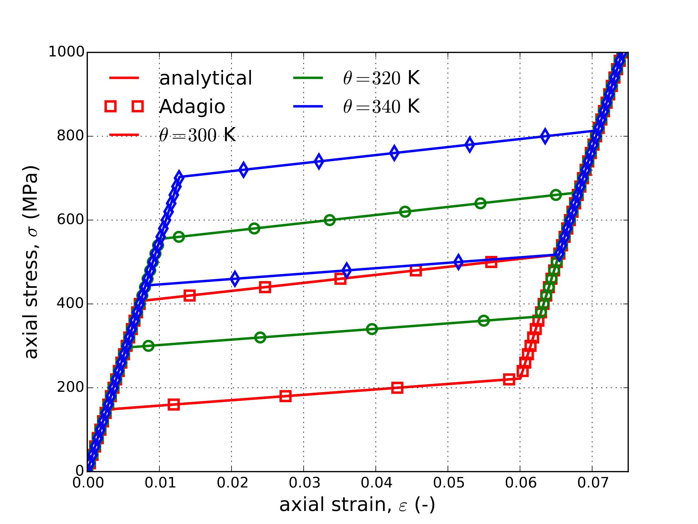
The results of this simple analytical expression and those determined by Adagio are presented in Fig. 4.118 for three different temperatures. Fig. 4.118(a) presents the stress-strain response under these conditions while Fig. 4.118(b) presents the evolution of the martensitic volume fraction.

Axial stress-strain

MVF

Fig. 4.118 Axial stress-strain response (a) and martensitic volume fraction (b), \(\xi\), evolution determined analytically and via adagio for three different ambient temperatures \(\theta=300,~320\) and \(340\) K.

4.25.3.2. Constant Stress Actuation

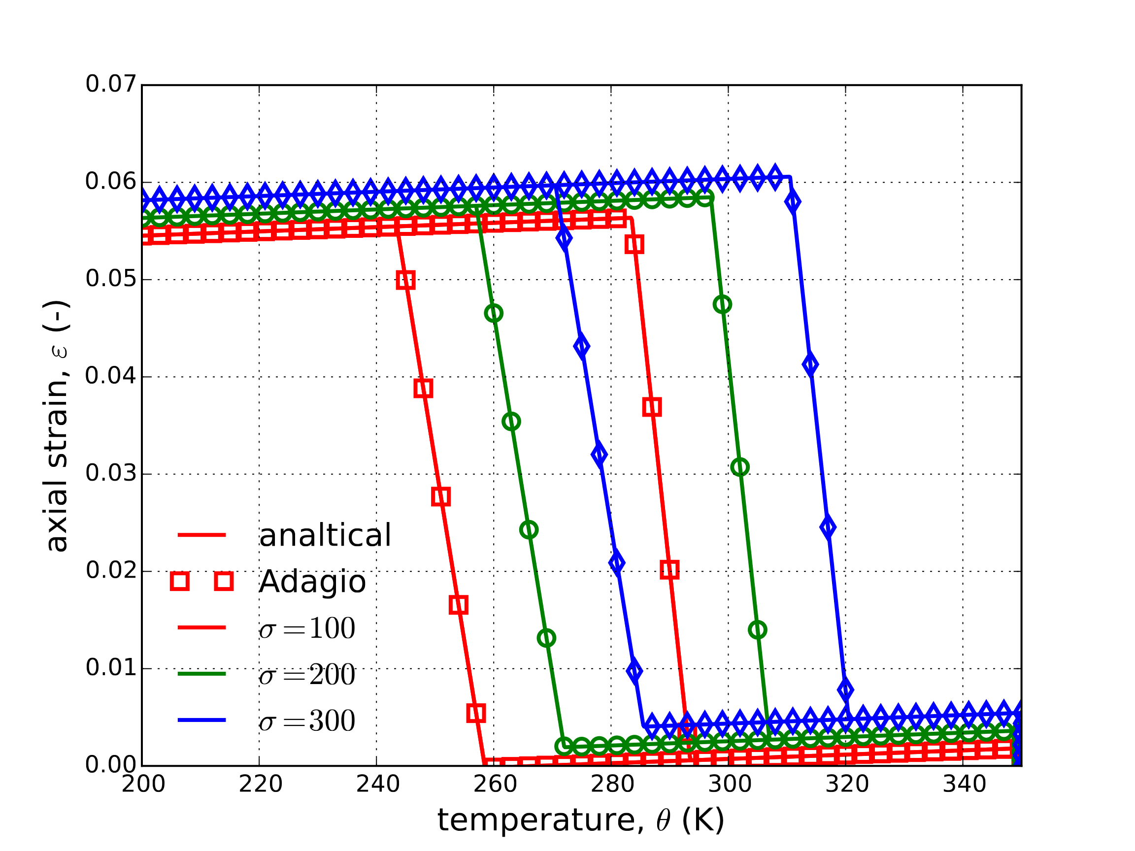
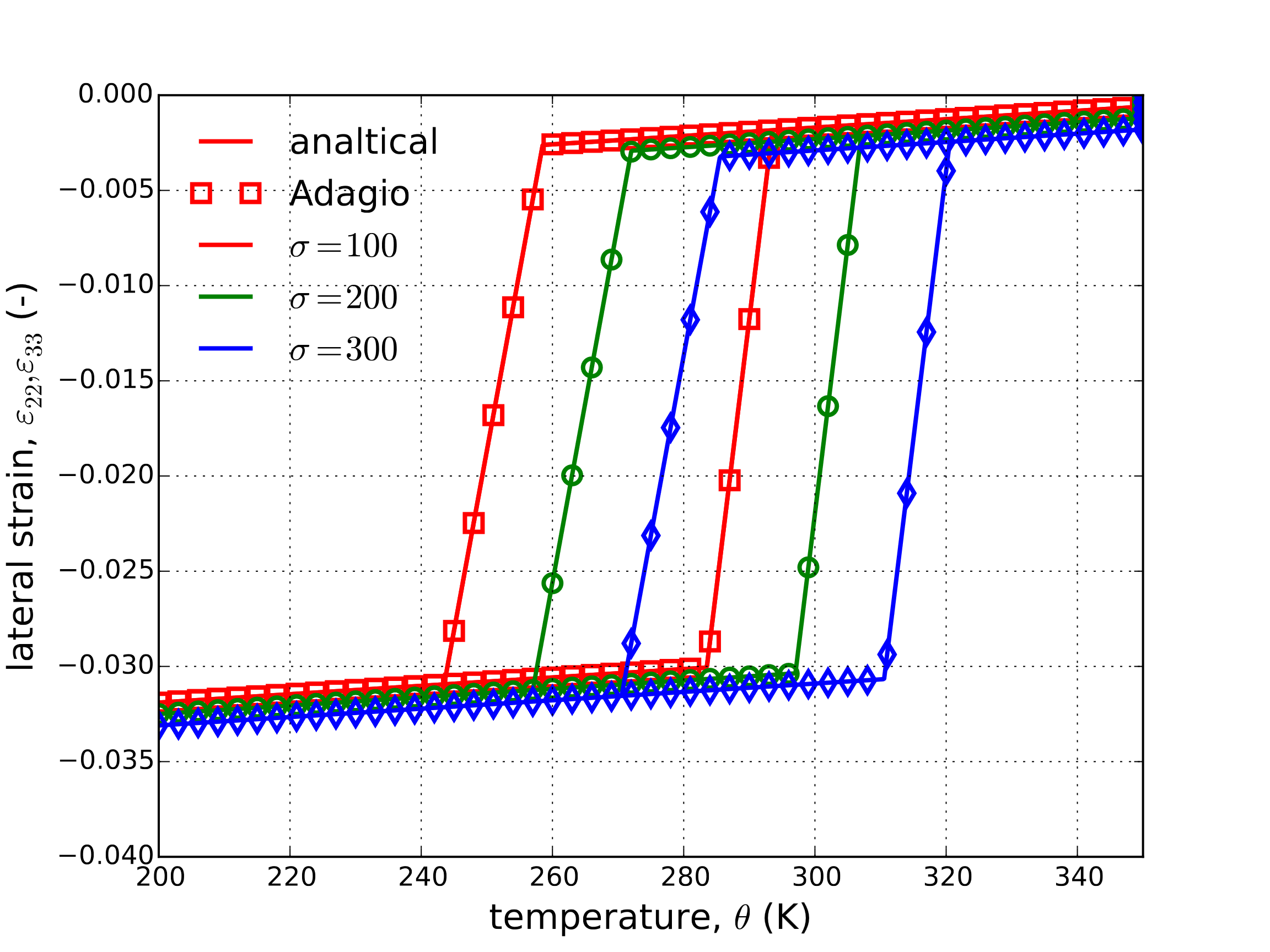
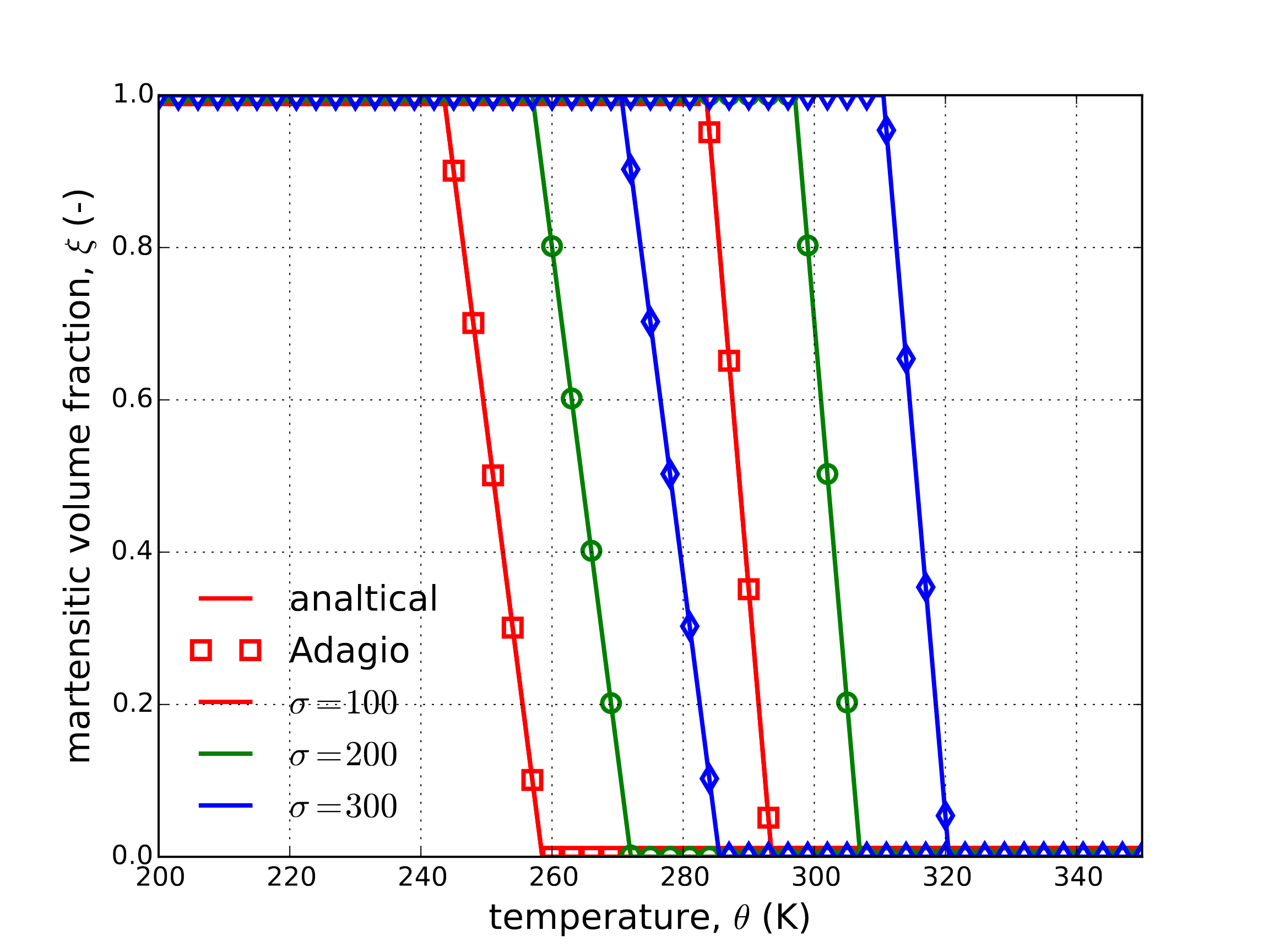
To consider thermally driven transformation, the constant stress actuation response is investigated. In such a loading, a mechanical load is applied at high temperature (\(\theta>A_f\)) and held constant while the specimen is cooled through forward transformation and then heated back to its initial state. Given the aforementioned simplifications to the model parameters, the analytical response is determined in a very similar fashion to that of pseudoelasticity. In this instance, critical temperatures needed for transformation are first determined by

\[\beta^{\sigma}=\beta + \frac{\sigma}{C},~\qquad \beta=M_s,~M_f,~A_s,~A_f,\]

with \(M_s^{\sigma}\) being the temperature needed to start forward transformation at an effective stress, \(\sigma\). The zero-stress value is \(M_s\). Similarly, the axial and lateral strains may be adjusted as,

\[\begin{split}\varepsilon_{11} & = \frac{\sigma}{E}+\xi H+\alpha\left(\theta-\theta_0\right), \\ \varepsilon_{22} = \varepsilon_{33} & = -\nu\frac{\sigma}{E}-\frac{1}{2}\xi H + \alpha\left(\theta-\theta_0\right).\end{split}\]

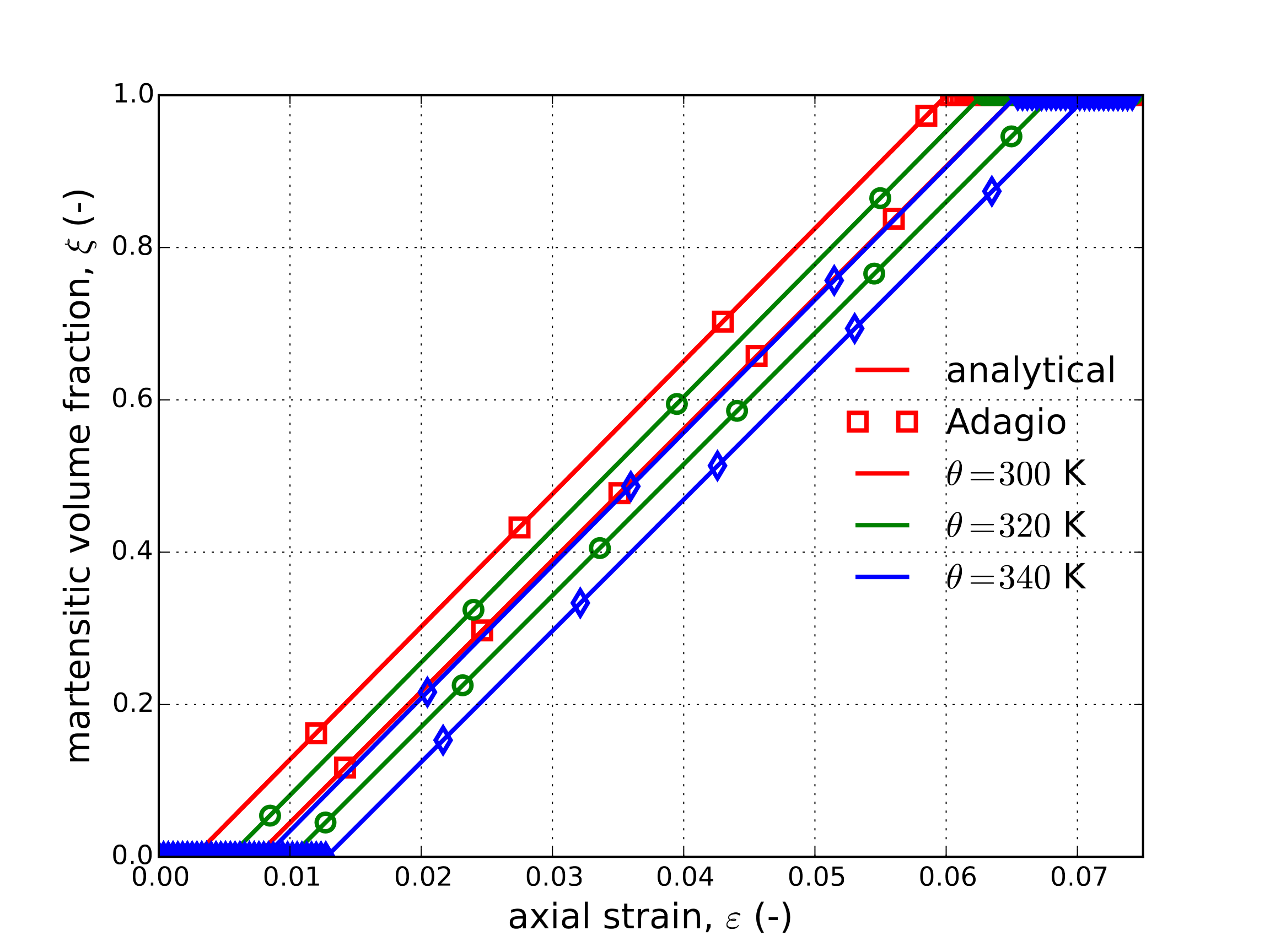
The martensitic volume fraction is found through relations (4.118) albeit with the piecewise intervals defined in terms of temperature (e.g \(\sigma^{Ms}<\sigma<\sigma^{M_f}~\leftrightarrow~M_f^{\sigma}<\theta<M_s^{\sigma}\)). Results for the axial strain-temperature, lateral strain-temperature, and martensitic volume fraction-temperature as determined analytically and via adagio are presented below in Fig. 4.119(a), Fig. 4.119(b), and Fig. 4.119(c), respectively.

Axial stress-strain

Laterial Strain

MVF

Fig. 4.119 Axial stress-strain (a), lateral strain (b), and martensitic volume fraction (c), \(\xi\), evolution as a function of temperature as determined analytically and numerically (Sierra/SM). Results are presented for three different applied bias stresses \(\sigma=100,~200\) and \(300\) MPa.

4.25.4. User Guide

BEGIN PARAMETERS FOR MODEL SHAPE_MEMORY_ALLOY
  #
  # Elastic constants
  #
  YOUNGS MODULUS = <real>
  POISSONS RATIO = <real>
  SHEAR MODULUS  = <real>
  BULK MODULUS   = <real>
  LAMBDA         = <real>
  TWO MU         = <real>
  #
  # Thermoelastic properties of two crystallographic phases
  #
  ELASTIC MODULUS AUSTENITE  = <real>
  POISSON RATIO AUSTENITE    = <real>
  CTE AUSTENITE              = <real>
  ELASTIC MODULUS MARTENSITE = <real>
  POISSON RATIO MARTENSITE   = <real>
  CTE MARTENSITE             = <real>
  #
  # Phase diagram parameters
  #
  MARTENSITE START                  = <real>
  MARTENSITE FINISH                 = <real>
  AUSTENITE START                   = <real>
  AUSTENITE FINISH                  = <real>
  STRESS INFLUENCE COEFF MARTENSITE = <real>
  STRESS INFLUENCE COEFF AUSTENITE  = <real>
  #
  # Transformation strain magnitude parameters
  #
  H_MIN          = <real>
  H_SAT          = <real>
  KT             = <real>
  SIGMA_CRITICAL = <real>
  #
  # Calibration parameters
  #
  N1         = <real>
  N2         = <real>
  N3         = <real>
  N4         = <real>
  SIGMA STAR = <real>
  T0         = <real>
  #
  # Initial phase conditions
  #
  XI0                 = <real> (0.0)
  PRESTRAIN_DIRECTION = <int> (0)
  PRESTRAIN_MAGNITUDE = <real> (0.0)
  #
END [PARAMETERS FOR MODEL SHAPE_MEMORY_ALLOY]

In the command blocks that define the Shape Memory Alloy model:

• Although the thermoelastic constants of the phases are defined separately, the definition of these constants in this form is necessary for the global solver. Typical values of the phases should be applied.

• The isotropic elastic moduli of the austenitic (\(E^A\)) and martensitic phases (\(E^M\)) are defined with the ELASTIC MODULUS AUSTENITE and ELASTIC MODULUS MARTENSITE command lines, respectively. Note, alternative elastic constants (e.g. bulk or shear moduli) may not be used.

• The isotropic Poisson’s ratio of the austenitic (\(\nu^A\)) and martensitic phases (\(\nu^M\)) are defined with the POISSON RATIO AUSTENITE and POISSON RATIO MARTENSITE command lines, respectively. Note, alternative elastic constants (e.g. lame constant) may not be used.

• The isotropic coefficient of thermal expansion of the austenitic (\(\alpha^A\)) and martensitic phases (\(\alpha^M\)) are defined with the CTE AUSTENITE and CTE MARTENSITE command lines, respectively. Note, given the phase and history dependence of the material thermal expansion, the use of artificial or thermal strain functions may not lead to desired results. The use of these constants in encouraged instead.

• The zero stress, smooth transformation temperatures corresponding to the start and end of forward transformation (martensitic start \(M_s\) and finish \(M_f\), respectively) and start and end of reverse transformation (austenitic start \(A_s\) and finish \(A_f\), respectively) are given by the (in order) command lines MARTENSITE START, MARTENSITE FINISH, AUSTENITE START, and AUSTENITE FINISH.

• The stress influence coefficients giving the slope of the forward and reverse transformation surfaces (\(C^M\) and \(C^A\), respectively) are given by the STRESS INFLUENCE COEFF MARTENSITE and STRESS INFLUENCE COEFF AUSTENITE, respectively.

• The stress dependence of the transformation strain magnitude requires four coefficients. These are the minimum transformation strain magnitude (\(H_{\text{min}}\)), the saturation (or maximum) magnitude (\(H_{\text{sat}}\)), exponential fitting coefficient (\(k\)), and critical effective stress value below which the magnitude is minimum (\(\sigma_{\text{crit}}\)). These parameters are defined via the H_MIN, H_SAT, KT, and SIGMA_CRITICAL command lines, respectively.

• The smooth hardening fitting constants \(n_1,~n_2,~n_3,\) and \(n_4\) correspond to the degree of smoothness (essentially how gradual the transformation is) of the martensitic start, martensitic finish, austenitic start, and austenitic finish transformation surfaces. They are given by the N1, N2, N3, and N4 command lines, respectively, and should take values \(0<n_i\leq 1\).

• The stress level of transformation at which calibration is performed is denoted by \(\sigma^*\) and given by the command line SIGMA STAR. For thermally induced transformation this corresponds to the bias stress level while in pseudo-elastic loadings it corresponds to the stress level at which the material is roughly evenly split between martensite and austenite.

• The zero-strain reference temperature is denoted \(\theta_0\) and prescribed via the T0 command line.

• Three optional parameters describing the initial state of the material may be input. These parameters are intended for the case in which the material is initially martensite to allow for initial heating and transformation recovery. The first is the initial martensitic volume fraction, \(\xi\left(t=0\right)\), input via the XI0 command line. If this parameter is not specified the default value is \(0.0\) representative of an austenitic material. A value between \(0.0\) and \(1.0\) may be entered to initialize the material to partially (or fully) martensitic. Corresponding initial transformation strains may be entered via the PRESTRAIN_DIRECTION \(\left(n^{\text{ps}}\right)\) and PRESTRAIN_MAGNITUDE \(\left(||\varepsilon^{\text{tr}}_{ij}\left(t=0\right)||\right)\) commands. The first (an integer between one and three) gives the direction of transformation (in global Cartesian space) and the magnitude of the inelastic strain in that direction is given by a fraction (between 0 and 1) of \(H_{\text{sat}}\) via the second PRESTRAIN_MAGNITUDE line. As the transformation strain tensor is deviatoric, the other two directions are specified by preserving that the tensor be trace less. Note, the PRESTRAIN_DIRECTION and PRESTRAIN_MAGNITUDE cannot be specified without a non-zero XI0 definition.

• Thermal strains functions and commands in Sierra should not be used in conjunction with the shape_memory_alloy model.

• In order for this material model to function a temperature must be defined on every block that uses the model.

Output variables available for this model are listed in Table 4.38.

Table 4.38 State Variables for SHAPE MEMORY ALLOY Model

Name	Description
MVF	martensitic volume fraction, \(\xi\)
TransStrain	transformation strain tensor, \(\varepsilon_{ij}^{\text{tr}}\)

---

[1] (1,2)

D. C. Lagoudas, editor. Shape Memory Alloys: Modeling and Engineering Application. Springer, New York, NY USA, 2008.

[2]

K. Otsuka and X. Ren. Physical metallurgy of Ti-Ni-based shape memory alloys. Progress in Materials Science, 50:511–678, 2005.

[3] (1,2,3)

D. Lagoudas, D. Hartl, Y. Chemisky, L. Machado, and P. Popov. Constitutive model for the numerical analysis of phase transformation in polycrystalline shape memory alloys. International Journal of Plasticity, 32-33:155–183, 2012.

[4]

D. J. Hartl, D. C. Lagoudas, F. T. Calkins, and J. H. Mabe. Use of a Ni60Ti shape memory alloy for active jet engine chevron application: I. thermomechanical characterization. Smart Materials and Structures, 19:015020, 2010.

[5]

D. J. Hartl, J. T. Mooney, D. C. Lagoudas, F. T. Calkins, and J. H. Mabe. Use of a Ni60Ti shape memory alloy for active jet engine chevron application: II. experimentally validated numerical analysis. Smart Materials and Structures, 19:015021, 2010.

[6]

M. A. Qidwai and D. C. Lagoudas. Numerical implementation of a shape memory alloy thermomechanical constitutive model using return mapping algorithms. International Journal for Numerical Methods in Engineering, 47:1123–1168, 2000.