4.11. Multilinear Elastic-Plastic Fail Model

4.11.1. Theory

Like the ductile fracture model, the multilinear elastic-plastic fail model is an extension of an existing plasticity model (multilinear elastic-plastic) to include a ductile failure criteria. Again, the tearing parameter criterion and failure propagation model of Wellman [[1]] is selected. Specifically, this approach uses a failure criterion (the tearing parameter, \(t_p\)) that is based on the history of the plastic strain and stress states. Most failure criteria for ductile failure involve some form of the stress triaxiality, or the ratio of the pressure and the effective (shear) stress. The tearing parameter, however, is slightly different in that it depends on the pressure and the maximum principal stress and is given as,

(4.37)\[t_p = \int_{0}^{\varepsilon} \left\langle\frac{2\sigma_{\text{max}}}{3\left(\sigma_{\text{max}}-\sigma_{m}\right)} \right\rangle^m d\varepsilon_{p},\]

with \(\sigma_{\text{max}}\) and \(\sigma_{m}\) being the maximum principal and mean stresses, respectively. The exponent \(m\) is typically taken to be 4 while the \(\langle \cdot \rangle\) are Macaulay brackets defined as,

\[\begin{split}\langle x \rangle = \left\{\begin{array}{cc} 0 & x \leq 0 \\ x & x > 0\end{array} \right. ,\end{split}\]

and introduced so that failure only occurs and propagates under tensile stress states. Failure then initiates when the tearing parameter, \(t_p\), reaches a critical value, \(t_p^{\text{crit}}\). After this point, the stress decays (to 0) in a linear fashion according to the ratio of the crack opening strain in the maximum principal stress direction to its critical value, \(\varepsilon_{\text{ccos}}\). Modification and control of this latter parameter is important as it may be used to ensure consistent energy is dissipated through different meshes.

4.11.2. Implementation

The multilinear elastic-plastic fail model seeks to capture both the nonlinear elastic-plastic and fracture responses of a ductile metal. Independently, each of these requirements necessitates the use of a nonlinear solution algorithm and the combination of the two is even more complex. This consideration is compounded by the relaxation and softening observed during the failure process that introduces additional complications for the global finite element solver. For this discussion, however, the focus is solely on the underlying numerical treatment of the failure process at the constitutive level. The solution of the elastic-plastic constitutive problem was discussed in detail in Section 4.10.2 while details of the implications at the global finite element problem are found in the Sierra/SM User’s Manual [[2]]. With respect to the latter, it is important to note that the ductile fracture model is tightly integrated with the multilevel CONTROL FAILURE capabilities although details of this coupling are left to [[1], [2]].

Prior to fracture initiation – while \(t_p^{n+1}<t_p^{\text{crit}}\) – the multilinear elastic-plastic fail model is the same as the “normal” multilinear elastic-plastic model. Through this process the tearing parameter is continually calculated at the plastically converged state. When fracture initiation is first detected – \(t_p^{n+1}\geq t_p^{\text{crit}}\) – the crack direction (assumed aligned with the maximum principal stress), denoted by the normalized vector \(n^{cr}_i\), is determined and stored. Regardless of loading path, this vector does not change during the unloading process. Additionally, for this first initial failure step, the unrotated stress tensor, \(T_{ij}\) must be updated to its maximum value, \(T_{ij}^{\text{crit}}\) before any unloading may be performed. This is done simply by,

\[T^{\text{crit}}_{ij}=T^n_{ij}+\left(T^{tr}_{ij}-T_{ij}^n\right)\frac{t_p^{\text{crit}}-t_p^n}{t_p^{n+1}-t_p^n},\]

with \(T^{tr}_{ij}\) being the elastic trial stress. As alluded to in the prior section, a linear decay based on the crack opening strain in the direction of maximum stress, \(\varepsilon_{\text{cos}}\), is utilized. To determine this decay value, the crack opening strain increment is first found via

\[d\varepsilon^{n+1}_{\text{cos}}=<\gamma n^{cr}_id^{n+1}_{ij}n^{cr}_j>,\]

where \(d^{n+1}_{ij}\) is the unrotated rate of deformation and \(\gamma\) is a partitioning factor between plastic and crack opening strains and takes the value of 1 for all loading steps except the initiation step and the “\(<\cdot>\)” are the Macaulay brackets. During the first fracture step,

\[\gamma=\frac{t_p^{n+1}-t_p^{\text{crit}}}{t_p^{n+1}-t_p^n}.\]

The current crack opening strain is then simply,

\[\varepsilon^{n+1}_{\text{cos}}=\varepsilon^n_{\text{cos}}+d\varepsilon^{n+1}_{\text{cos}}\Delta t.\]

and the decay factor, \(\alpha\), may be written as

\[\alpha^{n+1}=\max\left[0,\frac{\varepsilon_{\text{ccos}}-\varepsilon_{\text{cos}}^{n+1}}{\varepsilon_{\text{ccos}}}\right].\]

Given the temperature dependence, stress decay is slightly more complicated than in the ductile fracture case. This task is primarily accomplished by decreasing the yield stress (radius) proportionally with the decay factor,

\[\bar{\sigma}^{n+1}\left(\bar{\varepsilon}^{\text{p}}\right)=\alpha^{n+1}\bar{\sigma}^f,\]

where \(\bar{\sigma}^f=\phi\left(T^{\text{crit}}\right)\) is the yield stress at failure. The decayed stress is then found by radially returning to this reduced yield stress. Similarly, the hydrostatic and von Mises effective stress at failure (\(\sigma_m^f\) and \(\bar{\sigma}_{vM}^f\), respectively) are also calculated and stored to appropriately constrain the stress state. An additional check is then performed to ensure (and if necessary modify) the decayed stress to ensure that,

\[\sigma_m\leq\alpha\sigma_m^f; ~\qquad\qquad~ \bar{\sigma}_{vM}\leq\alpha\bar{\sigma}_{vM}^f.\]

4.11.3. Verification

The multilinear elastic-plastic model with failure has been tested with a number of verification tests. Specifically, uniaxial stress and uniaxial strain loadings are considered. For the elastic-plastic response, the same material properties as those in Section 4.10.3 are again considered. To this end, the Young’s modulus and Poisson ratio are \(E = 70\) GPa and \(\nu = 0.25\), respectively, and a Voce hardening model of the form,

\[\bar{\sigma}\left(\bar{\varepsilon}^p\right)=\sigma_y+A\left(1-\exp\left(-n\bar{\varepsilon}^p\right)\right),\]

is discretized and used. In this case, \(\sigma_y=200\) MPa, \(A = 200\) MPa, and \(n=20\).

In terms of failure, the critical tearing parameter, \(t_p^{\text{crit}}\) is taken to be .04, the critical crack opening strain, \(\varepsilon_{\text{ccos}}\), is .005 and \(m=4.0\).

4.11.3.1. Uniaxial Stress

To consider the uniaxial response, displacement controlled deformations are applied such that the only non-zero stress is the axial component, \(\sigma_{11}\). Through such a loading path, three distinct regimes result. The first is the elastic domain with \(t_p=0\). Second is the plastic domain. During this stage,

\[\sigma_{11}=\bar{\sigma}\left(\bar{\varepsilon}^p\right),\]

and by considering the rate of plastic work and integrating yields the implicit (in terms of equivalent plastic strain) relation,

\[\bar{\varepsilon}^p=\left(\varepsilon_{11}-\frac{\bar{\sigma}\left(\bar{\varepsilon}^p\right)}{E}\right).\]

By rearranging, the axial strain may be found in terms of the plastic strain as,

\[\varepsilon_{11}=\bar{\varepsilon}^p+\frac{\bar{\sigma}\left(\bar{\varepsilon}^p\right)}{E}.\]

With this stress state (\(\sigma_{ij}=\sigma_{11}\delta_{i1}\delta_{j1}\)), the pressure is simply \(\sigma_{11}/3\) and the maximum principal stress is \(\sigma_{\text{max}}=\sigma_{11}\). From (4.37), the tearing parameter is then

\[t_p=\bar{\varepsilon}^p.\]

The final stage of deformation corresponds to the failure process in which the axial stress is,

\[\sigma_{11}=\alpha\sigma_{\text{peak}},\]

and

\[\alpha=\frac{\varepsilon_{\text{ccos}}-\left(\varepsilon_{11}-\varepsilon_{\text{peak}}\right)}{\varepsilon_{\text{ccos}}}.\]

In the preceding relations, \(\sigma_{\text{peak}}\) and \(\varepsilon_{\text{peak}}\) are the axial stress and strain, respectively, at failure initiation. The former is simply \(\sigma_{\text{peak}}=\bar{\sigma}\left(t_p^{\text{crit}}\right)\) and \(\varepsilon_{\text{peak}}=t^{\text{crit}}_p+\sigma_{\text{peak}}/E\).

The tearing parameter and axial stress evolution as a function of axial strain are presented in Fig. 4.31(a) and Fig. 4.31(b), respectively. Good agreement is observed between the results verifying the model capability under such a loading. Three different numerical load incrementations were considered in this analysis and some dependence on load step is noted in the post-failure response of Fig. 4.31(b). Even with this observation, the resulting agreement between the different responses is still quite good.

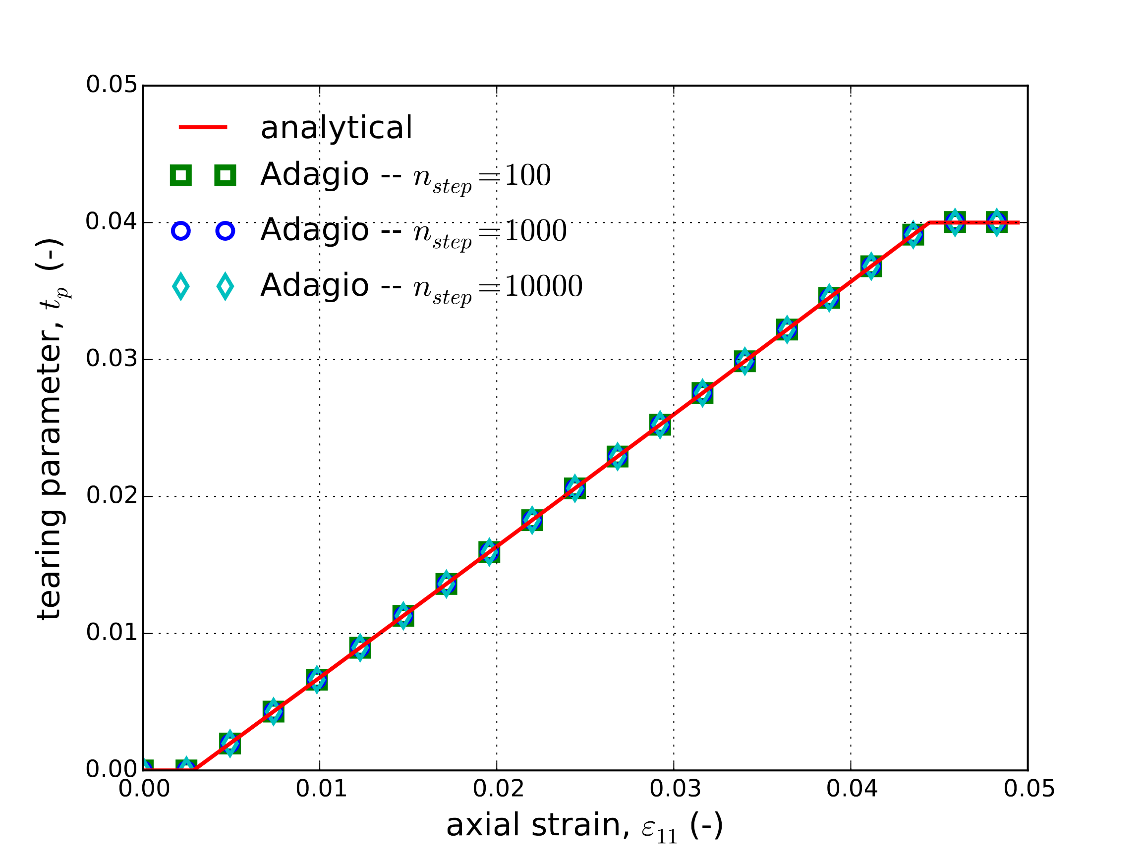
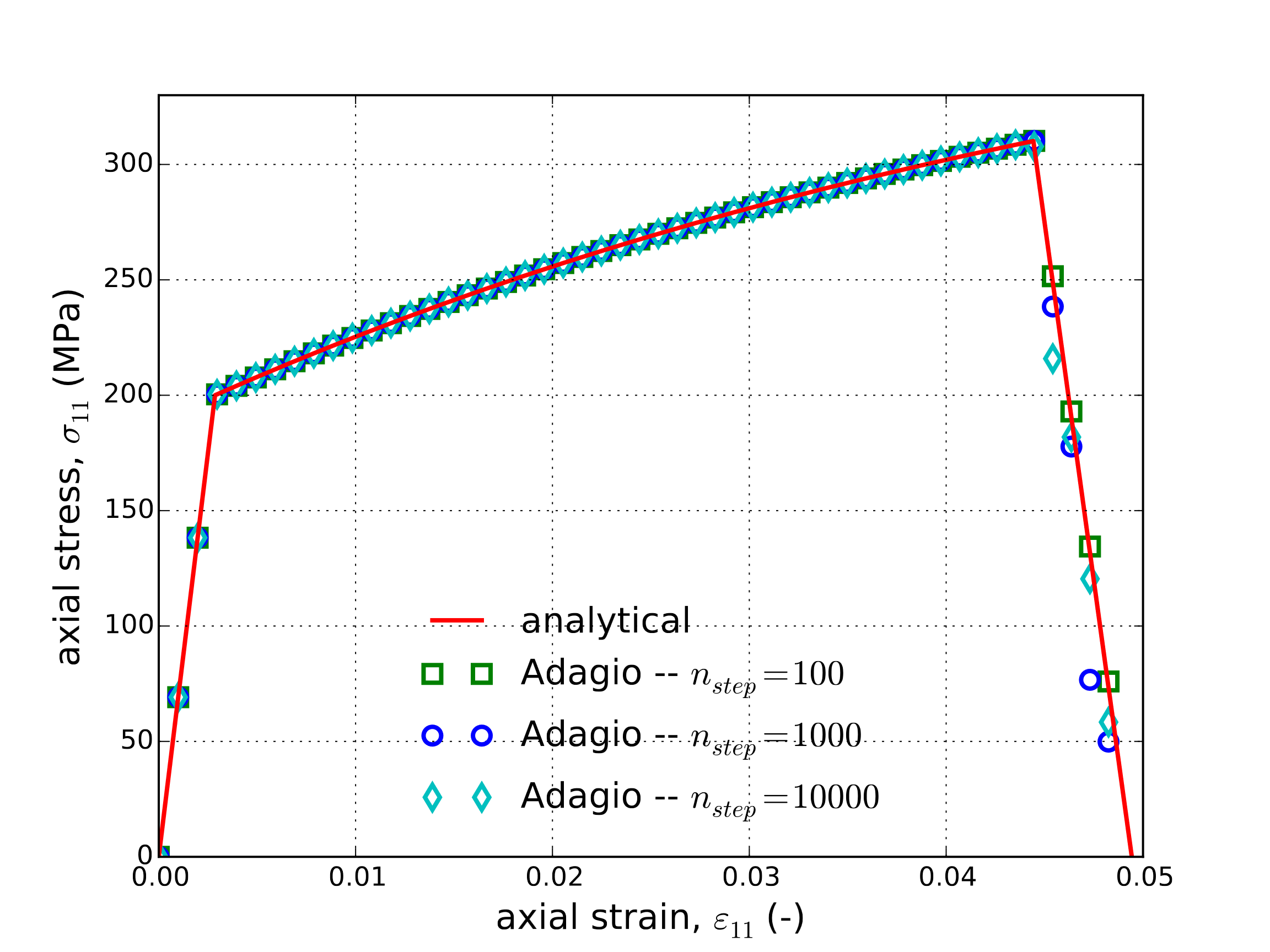
Fig. 4.31 Analytical and numerical results of the tearing parameter and axial stress evolution through a uniaxial tension loading path as a function of the axial strain, \(\varepsilon_{11}\).

4.11.3.2. Pure Shear

The analysis of the pure shear loading path follows closely with that of the ductile fracture model (Section 4.9.3.2). In this case, pure shear deformations are applied such that the only non-zero stress and strain are \(\sigma_{12}\) and \(\varepsilon_{12}\), respectively. Therefore, during plastic loading

\[\sigma_{12}=\frac{\bar{\sigma}}{\sqrt{3}},\]

and by comparing the plastic rate of work,

\[\varepsilon_{12}=\frac{\sqrt{3}}{2}\bar{\varepsilon}^p+\frac{\bar{\sigma}\left(\bar{\varepsilon}^p\right)}{\sqrt{3}\mu}.\]

Additionally, as the stress state is purely in shear there is no hydrostatic stress and the maximum principal stress is simply \(\sigma_{\text{max}}=\sigma_{12}\) leading to an expression for the tearing parameter of the form,

\[t_p=\left(\frac{2}{3}\right)^4\bar{\varepsilon}^p.\]

The stress then simply decays after the critical tearing parameter is reached. Numerical (from Adagio) and analytical results are presented in Fig. 4.32. Specifically, the tearing parameter and shear stress evolutions are presented in Fig. 4.32(a) and Fig. 4.32(b), respectively. Clear agreement is noted indicating the ability of the model to capture the response over a variety of loading paths.

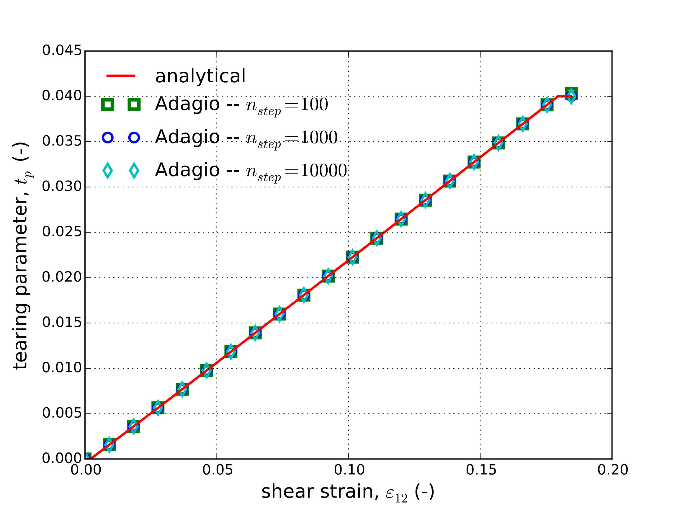
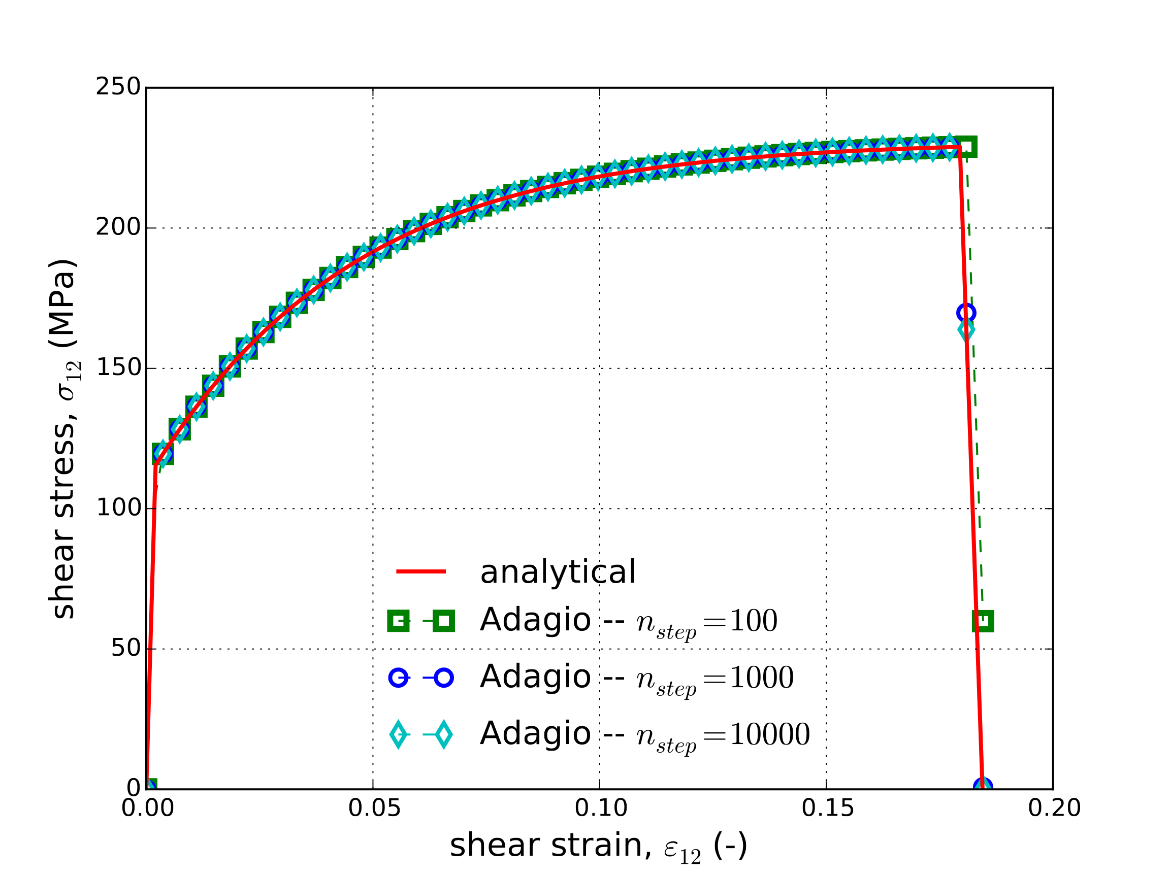
Fig. 4.32 Analytical and numerical results of the tearing parameter and shear stress evolution through a pure shear loading path as a function of the shear strain, \(\varepsilon_{12}\).

4.11.4. User Guide

BEGIN PARAMETERS FOR MODEL ML_EP_FAIL
  #
  # Elastic constants
  #
  YOUNGS MODULUS = <real>
  POISSONS RATIO = <real>
  SHEAR MODULUS  = <real>
  BULK MODULUS   = <real>
  LAMBDA         = <real>
  TWO MU         = <real>
  #
  # Hardening behavior
  #
  YIELD STRESS       = <real>
  BETA               = <real> (1.0)
  HARDENING FUNCTION = <string> hardening_function_name
  #
  # Functions
  #
  YOUNGS MODULUS FUNCTION = <string> ym_function_name
  POISSONS RATIO FUNCTION = <string> pr_function_name
  YIELD STRESS FUNCTION   = <string> yield_stress_function_name
  #
  # Failure parameters
  #
  CRITICAL TEARING PARAMETER    = <real>
  CRITICAL CRACK OPENING STRAIN = <real>
  CRITICAL BIAXIALITY RATIO     = <real> critical_ratio(0.0)
  FAILURE EXPONENT              = <real> (4.0)
END [PARAMETERS FOR MODEL ML_EP_FAIL]

In the above command blocks:

• The beta parameter defines if hardening is isotropic or kinematic.

• YIELD STRESS defines the stress for onset of yielding and plasticity.

• The HARDENING FUNCTION command line references the name of a function defined in a FUNCTION command line in the SIERRA scope. The function describes the hardening behavior of the material as stress versus equivalent plastic strain. The x values of the function should be values of equivalent plastic strain while the y values of the function can be either the increment of stress over the yield stress or the actual stress at the corresponding equivalent plastic strain. Note the hardening function can have its first point defined at (0,0), or at (0, YIELD_STRESS). Either function definition behaves the same as only the slope of the hardening function between two strains is used by the model.

• The YOUNGS MODULUS FUNCTION command line references the name of a function defined in a FUNCTION command line in the SIERRA scope that describes a scale factor on Young’s modulus as a function of temperature.

• The POISSONS RATIO FUNCTION command line references the name of a function defined in a FUNCTION command line in the SIERRA scope that describes a scale factor on Poisson’s ratio as a function of temperature.

• The YIELD STRESS FUNCTION command line references the name of a function defined in a FUNCTION command line in the SIERRA scope that describes a scale factor on the yield stress as a function of temperature.

• CRITICAL TEARING PARAMETER defines the \(t_{p}\) value at which fracture and subsequent decay of stress will occur.

• When the model undergoes additionally strain after reaching the critical tearing parameter the stress in the model will decay to zero. The amount strain over which the stress decays to zero is defined with the CRITICAL CRACK OPENING STRAIN command line. The relevant opening strain is the component of strain that is aligned with the maximum-principal-stress direction at initial failure.

• The CRITICAL BIAXIALITY RATIO command line should only be used under highly specific conditions and with extreme caution. It is intended only for the special case where the stress state is nearly biaxial, resulting in nearly identical principal strains. In this case, the eigenvector computation can give unreliable results for the direction vectors for the principal strains. If the ratio of the difference between two principal strains divided by their magnitude is less that the value specified by the CRITICAL BIAXIALITY RATIO command, the direction of the vector defining the crack opening strain will be given equal weight in each of the principal directions associated with those strains. The default value for the critical ratio is 0.0, which means that the principal directions will be accepted directly from the eigenvector computation. This command should only be used as a last resort if the loading is nearly biaxial and the default value has been demonstrated to lead to elements with high strains that are not failing long after reaching the critical tearing parameter.

• The FAILURE EXPONENT command line specifies the exponent on the tearing parameter, the m parameter in (4.37). This exponent defaults to 4.0.

Output variables available for this model are listed in Table 4.12 and Table 4.13.

Table 4.12 State Variables for ML EP FAIL Model

Name	Description
EQPS	Equivalent plastic strain
RADIUS	Radius of yield surface
BACK_STRESS	back stress - tensor
BACK_STRESS_XX	back stress - xx component
BACK_STRESS_YY	back stress - yy component
BACK_STRESS_ZZ	back stress - zz component
BACK_STRESS_XY	back stress - xy component
BACK_STRESS_YZ	back stress - yz component
BACK_STRESS_ZX	back stress - zx component
YOUNGS_MODULUS	Current Young’s modulus as a function of temperature
POISSONS_RATIO	Current Poisson’s ratio as a function of temperature
YIELD_STRESS	Current Yield stress as a function of temperature
TENSILE_EQPS	equivalent plastic strain only accumulated when the material is in tension (trace of stress tensor is positive)
ITERATIONS	radial return iterations
YIELD_FLAG	inside(0) or on(1) yield surface
TEARING_PARAMETER	Current integrated value of the tearing parameter. Zero until yield is reached
CRACK_OPENING_STRAIN	Current value of the crack opening strain. Zero until the critical tearing parameter is reached
FAILURE_DIRECTION	crack opening direction at failure - vector
FAILURE_DIRECTION_X	crack opening direction at failure - x component
FAILURE_DIRECTION_Y	crack opening direction at failure - y component
FAILURE_DIRECTION_Z	crack opening direction at failure - z component
MAX_RADIUS	maximum radius at initial failure
MAX_PRESSURE	maximum stress pressure norm at initial failure
CRITICAL_CRACK_OPENING_STRAIN
CRITICAL_TEARING_PARAMETER

Table 4.13 State Variables for ML EP FAIL Model for Shells

Name	Description
EQPS	equivalent plastic strain
RADIUS	radius of yield surface
BACK_STRESS	back stress - tensor
BACK_STRESS_XX	back stress - xx component
BACK_STRESS_YY	back stress - yy component
BACK_STRESS_ZZ	back stress - zz component
BACK_STRESS_XY	back stress - xy component
BACK_STRESS_YZ	back stress - yz component
BACK_STRESS_ZX	back stress - zx component
YOUNGS_MODULUS	Current Young’s modulus as a function of temperature
POISSONS_RATIO	Current Poisson’s ratio as a function of temperature
YIELD_STRESS	Current Yield stress as a function of temperature
ITER	radial return iterations
ERROR	Error in plane stress iterations
PS_ITER	Plane stress iterations
TEARING_PARAMETER	Current integrated value of the tearing parameter. Zero until yield is reached
CRACK_OPENING_STRAIN	Current value of the crack opening strain. Zero until the critical tearing parameter is reached
FAILURE_DIRECTION	crack opening direction at failure - vector
FAILURE_DIRECTION_X	crack opening direction at failure - x component
FAILURE_DIRECTION_Y	crack opening direction at failure - y component
FAILURE_DIRECTION_Z	crack opening direction at failure - z component
RADIUS_MAX	maximum radius at initial failure
TENSILE_EQPS	equivalent plastic strain only accumulated when the material is in tension (trace of stress tensor is positive)

---

[1] (1,2)

G. W. Wellman. A simple approach to modeling ductile failure. Technical Report SAND2012-1343, Sandia National Laboratories, Albuquerque, NM, June 2012. \href http://infoserve.sandia.gov/sand_doc/2012/121343.pdfpdf.

[2] (1,2)

Sierra/SolidMechanics Team. Sierra/SolidMechanics VOTD User’s Guide. Technical Report In draft, Sandia National Laboratories, Albuquerque, NM, 2019.