3.2.17. One-Dimensional Composite Fire Boundary Condition

3.2.17.1. Conceptual Overview

Fuego includes a boundary condition that is capable of modeling the thermal decomposition and outgassing of a thin sheet of porous material at the boundary surface, initially intended to simulate the combustion of a sheet of carbon fiber composite material. Variation through the material thickness is assumed to be locally one-dimensional. The actual implementation is quite flexible, allowing the simulation of the thermal response of essentially any finite-thickness material that can optionally undergo a user-specified chemical decomposition mechanism.

Figure 3.6 illustrates a two-dimensional representation of the virtual mesh used for this 1D composite fire boundary condition. One layer of elements above the boundary is shown, within which Fuego performs its normal fluid solve using the control volume finite element CVFEM method. The CVFEM sub-control volumes are demarcated with dashed lines. An equal-order interpolation methodology is used, so that all solution variables are stored at the element vertices.

For this boundary condition, a series of independent one-dimensional virtual domains exist behind each CVFEM surface node, and each virtual 1D domain has a cross-sectional area that matches the group of CVFEM boundary sub-control surfaces that contain the single “parent” surface node. A classical cell-centered finite volume methodology is used for the 1D virtual domains, where the discretization, storage, and numerical solutions all occur within the boundary condition implementation and only interact with the main CVFEM flow solution through fluxes and solution variables at the exposed surface.

Each 1D domain is assumed to have a fixed geometry that is filled with a simple porous material that is allowed to react chemically to form gaseous species. Since the overall volume of each element is fixed, the porosity of each volume is assumed to increase as species are converted from solid to gas. It is assumed that the gaseous species within the pores of the solid phase are of secondary concern, and as such no discrete transport equation is solved for them. The approximation is instead made that all gases generated within the porous material appear instantaneously at the surface of the material as a flux into the main fluid solution. It would be straightforward to solve additional transport equations for fluid flow within the porous material if that level of fidelity were to become necessary, as in the case of oxidative reactions where oxygen must diffuse through the exposed surface into the porous material before reactions may occur.

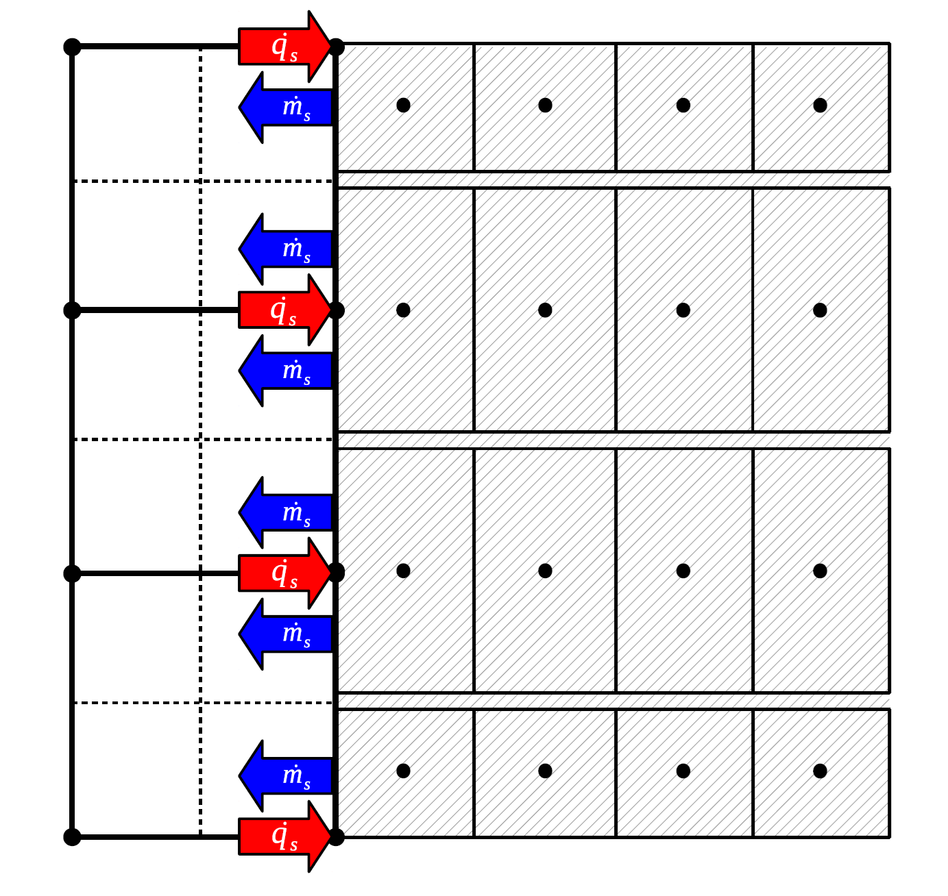
Fig. 3.6 Representative mesh layout for 1-D composite fire boundary condition

3.2.17.2. Model Formulation

3.2.17.2.1. Transport Equations

Within the solid phase of the porous material, one-dimensional transport equations for continuity, chemical species, and energy are solved in the form:

(3.504) $\pd{\bar{\rho}}{t} = \dot{\omega}_c'''$

(3.505) $\pd{\bar{\rho} Y_k}{t} = \dot{\omega}_k'''$

(3.506) $\bar{\rho} \bar{c} \pd{T}{t} = \pd{}{x} \left( \bar{k} \pd{T}{x} \right) + \dot{q}''',$

where $\bar{\rho}$ , $\bar{c}$ , and $\bar{k}$ are the mixture-averaged bulk density, specific heat, and thermal conductivity, respectively, $Y_k$ is the mass fraction of chemical species $k$ , $T$ is the temperature of the solid phase, $\dot{q}'''$ is the volumetric heat generation rate due to chemical reactions, $\dot{\omega}_k'''$ is the volumetric mass generation rate of chemical species $k$ , and $\dot{\omega}_c'''$ is the overall mass generation rate computed as $\dot{\omega}_c''' = \sum\limits_k \dot{\omega}_k'''$ .

3.2.17.2.2. Material Models

The composite material used for this boundary condition is assumed to be of a fixed volume, i.e. there is no structural deformation allowed. The bulk density of the multi-species solid mixture is assumed to be a function of the density of each component species in their native porous state, as

(3.507) $\bar{\rho} = \left( \sum\limits_k \frac{Y_k}{\rho_k} \right)^{-1},$

where $\rho_k$ is the porous density of species $k$ , provided as a material model by the user. This model for the mixture bulk density is only used to compute the initial bulk density field, which is subsequently solved directly from (3.504).

The porosity of the mixture is assumed to follow the model

(3.508) $\bar{\psi} = \sum\limits_k X_k \psi_k,$

where $X_k$ is the volume fraction of species $k$ ,

(3.509) $X_k = \bar{\rho} \frac{Y_k}{\rho_k},$

and $\psi_k$ is the porosity of pure species $k$ , modeled as

(3.510) $\psi_k = 1 - \frac{\rho_i}{\rho_{s0,k}},$

where $\rho_{s0,k}$ is the density of the solid (non-porous) species $k$ at a reference temperature. Note that the porosity does not appear explicitly in any of the transport equations or subsequent material models, so that it is never computed as part of the boundary condition solution. It would only appear in transport equations for the gaseous species occupying the pores of the solid skeleton, if this level of detail were ever to be added to this model.

In their most detailed form, the bulk thermal conductivity and specific heat are evaluated as a volume average and mass average of the individual species properties, respectively, as

(3.511) $\bar{k} = \sum\limits_k X_k k_k$

(3.512) $\bar{c} = \sum\limits_k Y_k c_k,$

although a species-independent model for the overall bulk property may be used if the individual species properties are not known.

The last quantities that require a model are the volumetric species mass production rates, $\dot{\omega}'''$ , and the volumetric heat production rate, $\dot{q}'''$ . These quantities can be provided by the user in two different ways. The traditional approach is to supply them using standard material property evaluations as a part of the material model definition. These are arbitrary functions that themselves may be dependent on any of the solution variables or other material properties. If a nonreacting material is desired, then these terms may be simply modeled as zero.

The second way of supplying these quantities is by including a chemistry description block in the material model, which allows the user to specify multiple reactions and variable composition gas production.

3.2.17.2.3. Boundary Conditions

The exposed surface of the composite material interacts thermally with the environment through several mechanisms, including convective heat transfer and both radiation absorption and emission. These external fluxes must balance the conduction inside the composite material at the surface, as

(3.513) $\dot{q}''' = \dot{q}'''_\mathrm{conv} + \dot{q}'''_\mathrm{rad}$

(3.514) $= \dot{q}'''_\mathrm{conv} + \epsilon \left(\sigma T_1^4 - \dot{q}'''_\mathrm{irr} \right)$

where $\dot{q}'''_\mathrm{conv}$ is the convective flux imposed on the surface by the external laminar or turbulent boundary condition treatment, $T_1$ is the temperature solution from the first control volume in the composite material used to model the gray emission, and $\dot{q}'''_\mathrm{irr}$ is the external radiative flux incident on the surface.

On the back-side of the virtual composite material, optional convective and radiative heat transfer to a quiescent environment is modeled as

(3.515) $\dot{q}'''_\mathrm{b} = \dot{q}'''_\mathrm{b,conv} + \dot{q}'''_\mathrm{b,rad}$

(3.516) $= h_c \left( T_N - T_\mathrm{ref} \right) + \sigma \epsilon_b \left(T_N^4 - T_\mathrm{ref}^4 \right)$

where $h_c$ is a user-specified convection coefficient, $\epsilon_b$ is a user-specified back-side emissivity, $T_\mathrm{ref}$ is the modeled ambient environment temperature, and $T_N$ is the temperature of the solution node closest to the back-side surface, assumed to be equal to the back-side surface temperature itself.

3.2.17.2.4. Numerical Implementation - Original

A segregated, implicit solution technique is used to numerically integrate (3.504)–(3.506). The discretized form of the continuity equation, (3.504), is derived by first integrating it over the finite volume $V$ and the time step $\Delta t$ to yield

(3.517) $\int_{\Delta t} \left[ \int_V \pd{\bar{\rho}}{t} dV - \int_V \dot{\omega}'''_c dV \right] dt = 0$

(3.518) $\int_{\Delta t} \left[ V_i \pd{\bar{\rho}_i}{t} - V_i \dot{\omega}'''_{c,i} \right] dt = 0.$

Discretizing the temporal derivative using a first-order backward difference approximation and solving for the bulk density at the new time step yields

(3.519) $V_i \left( \bar{\rho}_i^{n+1} - \bar{\rho}_i^n \right) - V_i \dot{\omega}_{c,i}''' \Delta t = 0$

(3.520) $\bar{\rho}_i^{n+1} = \bar{\rho}_i^n + \dot{\omega}_{c,i}''' \Delta t.$

where the mesh indices are defined in Figure 3.7. Note that this equation is linearized by evaluating the source term at the most recent estimate of the $n+1$ solution state.

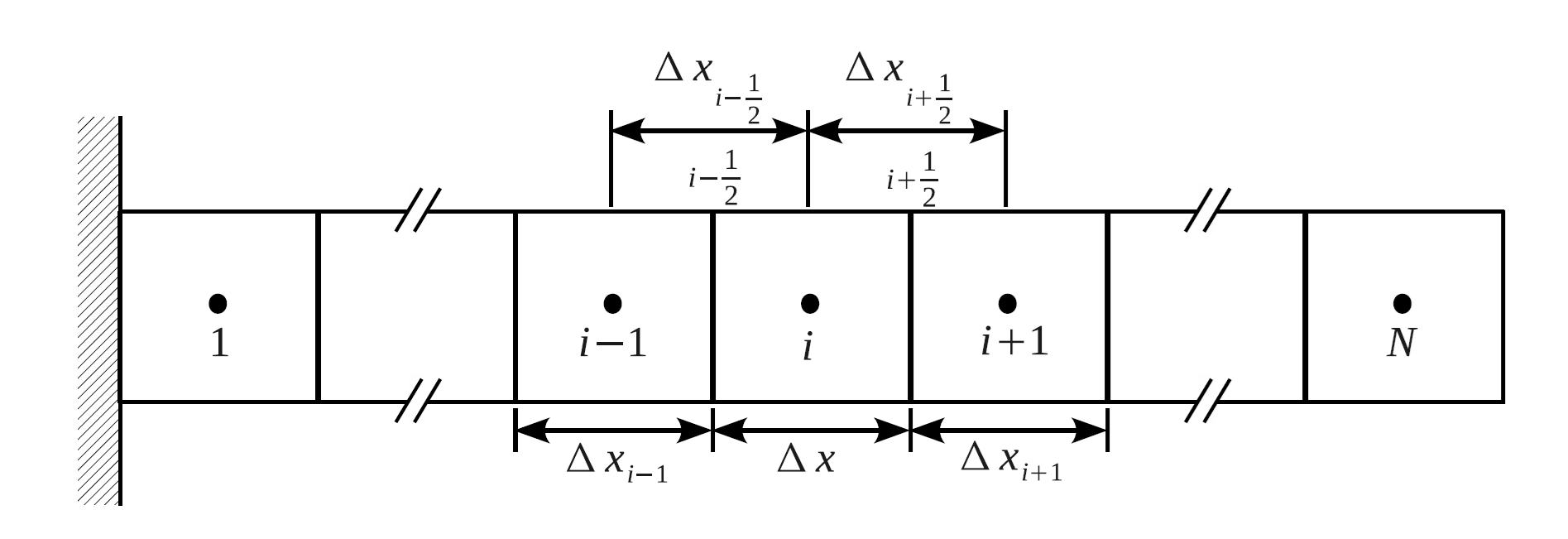
Fig. 3.7 Mesh index definition for 1-D composite fire boundary condition

The species transport equations, (3.505), undergoes an identical transformation,

(3.521) $\int_{\Delta t} \left[ \int_V \pd{\bar{\rho} Y_k}{t} dV - \int_V \dot{\omega}'''_k dV \right] dt = 0$

(3.522) $\int_{\Delta t} \left[ V_i \pd{\bar{\rho}_i Y_k}{t} - V_i \dot{\omega}'''_{c,i} \right] dt = 0.$

(3.523) $V_i \left( \bar{\rho}_i^{n+1} Y_{k,i}^{n+1} - \bar{\rho}_i^n Y_{k,i}^n \right) - V_i \dot{\omega}_{k,i}''' \Delta t = 0$

(3.524) $Y_{k,i}^{n+1} = \frac{ \bar{\rho}_i^n Y_{k,i}^n + \dot{\omega}_{k,i}''' \Delta t }{ \bar{\rho}_i^{n+1} },$

where the bulk density at the new time level is used from (3.520), and the source term is evaluated from the most recent estimate of the $n+1$ solution state.

The energy equation also undergoes a similar transformation, but with added complexity due to the inclusion of spatial derivatives. (3.506) is first integrated in both space and time, and the Gauss divergence theorem is used to remove one level of spatial derivatives in the diffusive flux term,

(3.525) $\int_{\Delta t} \left[ \int_V \bar{\rho} \bar{c} \pd{T}{t} dV - \int_V \pd{}{x} \left( \bar{k} \pd{T}{x} \right) dV - \int_V \dot{q}''' dV \right] dt = 0$

(3.526) $\int_{\Delta t} \left[ \int_V \bar{\rho} \bar{c} \pd{T}{t} dV - \int_A n \cdot \left( \bar{k} \pd{T}{x} \right) dA - \int_V \dot{q}''' dV \right] dt = 0.$

Integrating numerically in space yields

(3.527) $\int_{\Delta t} \left[ \bar{\rho}_i \bar{c}_i V_i \pd{T_i}{t} - \left( \left( - A \bar{k} \pd{T}{x} \right)_{i-\frac{1}{2}} + \left( A \bar{k} \pd{T}{x} \right)_{i+\frac{1}{2}} \right) - \dot{q}'''_i V_i \right] dt = 0$

(3.528) $\int_{\Delta t} \left[ \bar{\rho}_i \bar{c}_i V_i \pd{T_i}{t} + A_{i-\frac{1}{2}} \bar{k}_{i-\frac{1}{2}} \left( \frac{T_i - T_{i-1}}{\Delta x_{i-\frac{1}{2}}} \right) - A_{i+\frac{1}{2}} \bar{k}_{i+\frac{1}{2}} \left( \frac{T_{i+1} - T_i}{\Delta x_{i+\frac{1}{2}}} \right) - \dot{q}'''_i V_i \right] dt = 0,$

and then integrating in time and linearizing the equation by evaluating the coefficients at the most recent estimate of the $n+1$ solution state yields

(3.529) $\bar{\rho}_i \bar{c}_i V_i \left( \frac{T_i^{n+1} - T_i^n}{\Delta t} \right) + A_{i-\frac{1}{2}} \bar{k}_{i-\frac{1}{2}} \left( \frac{T_i^{n+1} - T_{i-1}^{n+1}}{\Delta x_{i-\frac{1}{2}}} \right) - A_{i+\frac{1}{2}} \bar{k}_{i+\frac{1}{2}} \left( \frac{T_{i+1}^{n+1} - T_i^{n+1}}{\Delta x_{i+\frac{1}{2}}} \right) - \dot{q}'''_i V_i = 0.$

This leads to a tri-diagonal system of coupled linear equations for the temperature at time level $(n+1)$ , which is solved using a direct method with the DGTSL module of the SLATEC library.

The continuity, species, and energy equations are solved sequentially in the order described, and the solution is repeated until the maximum normalized change in the temperature solution,

(3.530) $T_\mathrm{err} = \frac{ \left| T^{n+1} - T^* \right| }{ T^{n+1} }$

satisfies the user-specified tolerance, where $T^*$ is the solution from the previous iteration.

Please see the Fuego user’s manual for details on the usage of this boundary condition.

3.2.17.2.5. Numerical Implementation - New

When using the new form of the composite BC, where the chemical mechanism is specified using a chemistry description, the numerical implementation is slightly different. The finite volume discretization used is the same, but the system of equations is solved monolithically using the user-specified ODE solver. The solver handles time stepping during the sub-integration to reduce the overall error below the specified threshhold.

Additionally, when constructing the monolithic system with the new form the DOFs are temperature and $N$ species masses, rather than the prior approach of using temperature, density, and $N-1$ species mass fractions.