4.4.1.1. Enclosure Radiation
As described here, enclosure radiation accounts for radiative heat transfer
between surfaces of an enclosure wherein the intermediate medium is transparent. Modeling of enclosure radiation requires
determination of the energy transport between all  surface facets that comprise the enclosure, an
  description of
global interactions. Since direct coupling of the radiosity problem with the volume energy equations
would result in a monolithic solve, the approached used in Aria is instead to solve the enclosure radiation and volume energy equations (as well as any other equations that may appear in the equation system) independently but coupled through boundary conditions. Specifically, the enclosure radiation problem results in the following three main steps:
description of
global interactions. Since direct coupling of the radiosity problem with the volume energy equations
would result in a monolithic solve, the approached used in Aria is instead to solve the enclosure radiation and volume energy equations (as well as any other equations that may appear in the equation system) independently but coupled through boundary conditions. Specifically, the enclosure radiation problem results in the following three main steps:
Compute the viewfactors (if needed) or read in pre-computed viewfactors (if requested)
Solve the radiosity equation (3.114) using the current average facet temperature to compute a known RHS
Solve the linearized equation system for the temperature correction (as well as other DOF corrections) using the updated radiative heat flux (3.115) contribution and correct the temperature.
where the viewfactor step occurs prior to the nonlinear loop, whereas the last two steps repeat until the specified nonlinear convergence criteria is met.
Note
A given enclosure can be coupled through its surfaces to multiple energy equation types (e.g. EQ ENERGY, EQ POROUS_ENTHALPY), that may belong
to different equation systems. When this occurs, the viewfactor computation and radiosity solve are only performed in the first
(input deck order) segregated equation system that is coupled to the enclosure. As a result, the radiosity solve specified
by (3.114) will use lagged facet temperatures from other equation systems which will result in lagged radiosities
and correspondingly a lagged radiative flux will be applied. To avoid this, it is recommended that respective equations
are all defined in a single equation system.
The input deck below shows the incremental change needed to add an enclosure.
Begin Sierra myJob

  ...

  Begin Global Constants
    Stefan Boltzmann Constant = 5.6704e-08  # W/m2-K4
  End

  Begin Aria Material my_material
    # Define emissivity model
    emissivity = constant value = 1.0
    ...
  End

  Begin Procedure My_Aria_Procedure
    ...
    Begin Aria Region My_Region
      ...

      # Define the enclosure
      Begin Enclosure Definition enc1
        add surface surface_1 surface_2

        # Uncommenting will override the above emissivity model
        # emissivity = 0.5 on surface_1
        # emissivity = 0.6 on surface_2

        Use Viewfactor Calculation vf_calc
        Use Viewfactor Smoothing no_smooth
        Use Radiosity Solver Rad_Solv
      End

      # Define how the viewfactor is calculated
      Begin Viewfactor Calculation vf_calc
        Compute Rule            = Hemicube
        ...
      End

      # Define viewfactor smoothing
      Begin Viewfactor Smoothing no_smooth
        Method                = none
        ...
      End

      # Define solver to use for the radiosity equation
      Begin Radiosity Solver Rad_Solv
        Solver                  = chaparral GMRES
        Convergence Tolerance   = 1e-8
        Maximum Iterations      = 300
        ...
      End
      ...

      postprocess average of expression irradiance on surface_1 as G_avg
      postprocess average of expression rad_flux on surface_1 as q_avg
      postprocess average of expression radiosity on surface_1 as J_avg

      # Define enclosure facet field variables for output
      Begin Results Output Label encl_rad
        ...
        # in 2D, these are edge variables
        face variables = radiosity as J
        face variables = rad_flux as q
        face variables = irradiance as G
        face variables = emissivity as e
        face variables = face_temperature as T
      End
    End
  End
End Sierra myJob
To start, an enclosure definition command block defines the surfaces of the enclosure. These surfaces are automatically coupled
to respective volume energy equations through a radiative heat flux contribution. On these surfaces, several enclosure specific face field variables
are available for output, these include the rad_flux (3.115), irradiance (3.111), radiosity (3.109), emissivity, and face_temperature (3.110).
As shown above, expressions for the rad_flux, irradiance, and radiosity are also provided so that reductions operations can be performed.
Note
A dirichlet boundary condition for temperature specified on one of the enclosure surfaces will override any flux contribution from the enclosure to that surface. The radiosity equation will still be coupled to this surface through its right hand side term.
Specification of enclosure surfaces can either be done directly by enumerating the surfaces as shown above or alternatively, when used with the dash enclosures capability, by specifying a combination of volume blocks to skin and surfaces to include.
Warning
By default, if an enclosure surface touches a volume block that only has EQ POROUS_ENTHALPY in either the solid phase or gas phase,
the radiative flux will only contribute to the solid phase. When it is ambiguous which energy equation to couple the enclosure to,
an error will be thrown. To resolve the error, the matched flux line command must be used to
specify which equation should receive the radiative heat flux.
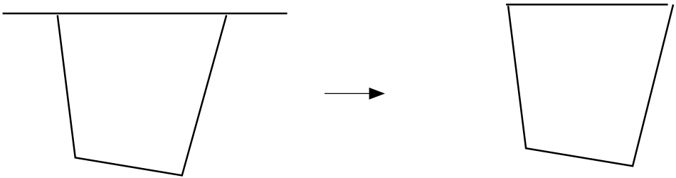
Fig. 4.8 Discretization and Associated Closed Enclosure Surface.
In all cases, the enclosure is viewed as a closed surface. As illustrated in Fig. 4.8 the discretization may need to be modified in order to properly define the closed surface. For problems in which the enclosure surface is not entirely meshed, it can be implicitly closed by defining a partial enclosure with appropriately defined properties specified within the enclosure definition command block.
As shown in the example input deck, within each enclosure definition command block, line commands reference separate command blocks that provide details concerning the viewfactor calculation, viewfactor smoothing, and radiosity solver.
Note
Line commands can be also used to define the emissivity for a particular surface in the enclosure definition command block. When the emissivity has been provided both from the block material (as shown above) and surface material, the surface material will override.
With respect to the viewfactor calculation, we have specified the most common approach i.e., the hemicube method. Details regarding the hemicube method are provided in [19]. The viewfactor command reference details additional line commands relevant to the hemicube method. If the same geometric model will be used for different analyses, saving the viewfactors to file and reading them in is recommended to reduce simulation time. This can be accomplished by first saving the viewfactors to a file via a command in the enclosure definition command block and then in a subsequent run changing the compute rule to read in the specified viewfactors e.g.
Begin Enclosure Definition enc1
  ...
  database name is viewfactors.vf in pnetcdf format
End

Begin Viewfactor Calculation vf_calc
  compute rule = read
  ...
End
Note
If no viewfactor file is found, the compute rule will default to the hemicube method. A message will be printed to the log indicating that viewfactors are being computed as opposed to read.
With respect to viewfactor smoothing, the above example uses none; however,
complex enclosures often require smoothing of the viewfactors
to ensure the quality of the viewfactors before proceeding to the radiosity solve.
One measure of how accurately the viewfactors are being computed
is the rowsum value. For each surface facet  in a fully-closed enclosure
the rowsum value should approach one i.e.,
in a fully-closed enclosure
the rowsum value should approach one i.e.,  , thus the total rowsum value
is always the number of facets. In cases where the target rowsum
is not equal to one the surface may not be fully-closed or the
viewfactor calculation may be inaccurate for some other reason.
In either event the analyst should investigate possible
causes of the discrepancy. Viewfactor smoothing may offset some of the errors
indicated by the rowsum values. The viewfactor smoothing command reference can be found
here.
, thus the total rowsum value
is always the number of facets. In cases where the target rowsum
is not equal to one the surface may not be fully-closed or the
viewfactor calculation may be inaccurate for some other reason.
In either event the analyst should investigate possible
causes of the discrepancy. Viewfactor smoothing may offset some of the errors
indicated by the rowsum values. The viewfactor smoothing command reference can be found
here.
Note
The viewfactor between two facets is
roughly proportional to  where
where  is the distance between
facet centroids. Thus it follows directly that facets which are
nearly parallel and opposing may adversely affect the viewfactor calculation.
Similar statements apply to poorly equivalenced surface intersections
leading to slivered surfaces becoming part of an enclosure.
In the worst of circumstances the viewfactor will simply fail
when the distance between facets is too small and the mesh may need to
be repaired.
is the distance between
facet centroids. Thus it follows directly that facets which are
nearly parallel and opposing may adversely affect the viewfactor calculation.
Similar statements apply to poorly equivalenced surface intersections
leading to slivered surfaces becoming part of an enclosure.
In the worst of circumstances the viewfactor will simply fail
when the distance between facets is too small and the mesh may need to
be repaired.
The above example outlines input commands blocks for enclosure radiation problems that are independent of the wavelength. When considering the wavelength dependence, a banded wavelength model can be used. This requires specifying additional command blocks as discussed here.
Note
For most cases the enclosure is devoid of
interior mesh discretization. In the event that the enclosure interior is meshed,
the interior mesh can be ignored by using the OMIT_VOLUME command line in the FINITE_ELEMENT_MODEL command block.
In the event one might require the interior mesh to represent other
coupled physics within the cavity area of the enclosure, the MESHED_ENCLOSURE command
can be specified in the enclosure definition command block to exclude the meshed block (and its surface) from the enclosure radiation problem.
For simulations in which enclosure radiation approaches the optically-thick
limit one might consider utilizing a meshed enclosure in conjunction with
the OPTICALLY\_THICK thermal conductivity model in lieu
of the enclosure radiation problem.
A full command reference for the various relevant line commands for all enclosure radiation command blocks is available here.
4.4.1.1.1. Partial Enclosures
When an enclosure is not entirely meshed, partial enclosures can be used to “close” the enclosure through a far field radiating condition. An example partial enclosure is demonstrated in Fig. 4.9.
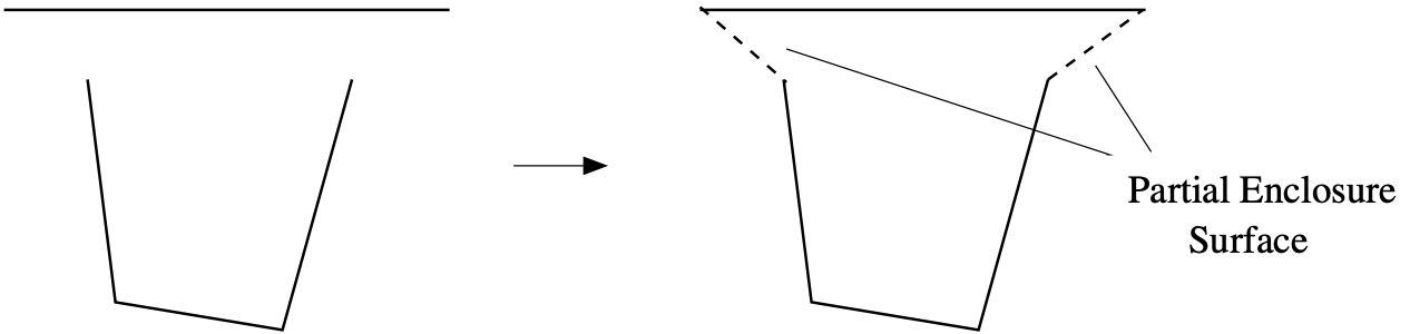
Fig. 4.9 Discretization and Associated Partial Enclosure Surface
Warning
It is important to ensure that the partial enclosure is properly formed and that unintended gaps are not included in the virtual partial surface. Notably, partial enclosures do not have row sum errors. As such, forgetting to include a surface or having a mesh defect will result in unintended energy leakage. Lastly, viewfactor smoothing can not be applied with partial enclosures as it will lead to erroneous viewfactors.
The concept of a partial enclosure is best demonstrated by use of a simplified view of radiative
transfer system between surfaces  and
and  surrounded by free space as shown in Fig. 4.10.
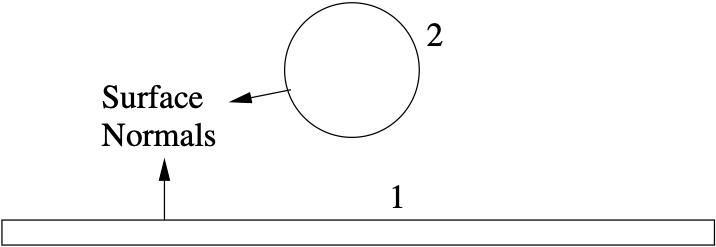
Fig. 4.10 Two-Body Radiative Transfer Model.
If radiative transfer occurs between the two bodies and the viewfactor between the two bodies is readily accessible a simplified network representation of the interaction, Fig. 4.11 may suffice but here the interest lies in analyzing the system using enclosure radiation.
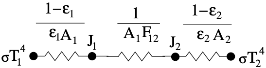
Fig. 4.11 Two Surface Network Model.
In many cases a more complete model of the two-body configuration will include radiative transfer with the surroundings. Including these interactions requires introduction of an additional enclosure surface as shown in Fig. 4.12.
Surface  known as the “partial enclosure” is artificially added to the
numerical model (i.e. not included in the meshed discretization). Introduction
of the partial enclosure is necessary in order to apply conventional approaches
for numerical evaluation of the system viewfactors. Here we note that
algorithmically, failure to add the partial enclosure surface would be manifest
in bad row-sum metrics.
known as the “partial enclosure” is artificially added to the
numerical model (i.e. not included in the meshed discretization). Introduction
of the partial enclosure is necessary in order to apply conventional approaches
for numerical evaluation of the system viewfactors. Here we note that
algorithmically, failure to add the partial enclosure surface would be manifest
in bad row-sum metrics.
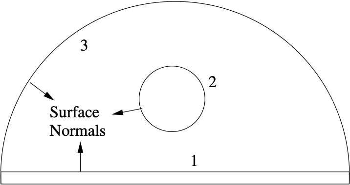
Fig. 4.12 Partial Enclosure Radiative Transfer Model.
Introduction of the partial enclosure leads to the thermal network representation shown in Fig. 4.13 in which the partial enclosure interacts with the other bodies of the system.
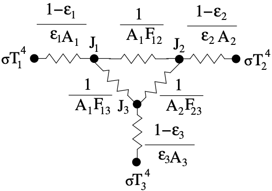
Fig. 4.13 Three Surface Network Model.
Since the partial enclosure is modeled in the same way as a real surface,
questions often arise concerning characterization of the partial enclosure in
terms of its temperature, area and emissivity. The temperature must of course
must represent the surroundings. The area should be an area that envelopes the
true surfaces of the enclosures. The partial enclosure emissivity should be
chosen in a manner consistent with the relationship of surface radiosity  with the emission,
  and irradiance,
  i.e.,
i.e.,
(4.5)
As examples of this we consider the consequence of selecting a partial
emissivity at two extremes,  and
and  , both of
which reduce the network model of Fig. 4.13 to that of
Fig. 4.14.
, both of
which reduce the network model of Fig. 4.13 to that of
Fig. 4.14.
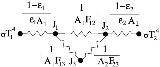
Fig. 4.14 Three Surface Network Model (

 ).
).
For from the network interaction between  we find that the resistance becomes infinite thus eliminating any system
interaction with
we find that the resistance becomes infinite thus eliminating any system
interaction with  as all the incident energy is reflected. This results
in a modified version of the two-surface network
Fig. 4.11, albeit with more attenuation. For
and the network interaction between is eliminated.
However, now the radiative transfer system sees the emissive power of the surroundings since from (4.5),
as all the incident energy is reflected. This results
in a modified version of the two-surface network
Fig. 4.11, albeit with more attenuation. For
and the network interaction between is eliminated.
However, now the radiative transfer system sees the emissive power of the surroundings since from (4.5),
 . Clearly there are no obvious choices for partial enclosure emissivity
other than that it should be chosen to enable interaction of the system with the
surroundings.
. Clearly there are no obvious choices for partial enclosure emissivity
other than that it should be chosen to enable interaction of the system with the
surroundings.
As part of the partial enclosure description one must supply a partial enclosure area. For many problems it may be difficult to initially compute or even estimate the partial enclosure area. For these cases provision is made within Aria to internally compute the minimum area that should be used. To obtain the minimum area one temporarily assigns a small number for the partial enclosure, starts the problem and terminates it after one step. The minimum partial enclosure area will be printed to the Chaparral log.
Note
The partial enclosure modifies the radiosity equation by one row and column with the partial
enclosure properties used to compute matrix entries and the right hand side entry.
For instance, the partial enclosure area determines the last row of viewfactors  via
the viewfactor reciprocity relation i.e.,
via
the viewfactor reciprocity relation i.e.,  , where
the last column of viewfactors
, where
the last column of viewfactors  are derived from the row sum relation i.e., .
Once the partial enclosure area, temperature and emissivity have been determined, they can be specified in the enclosure definition command block as follows
Begin Enclosure Definition enc1
  ...
  # Define partial enclosure
  partial enclosure area = 1.5738
  partial enclosure temperature = 293.0
  partial enclosure emissivity = 1.0

  # Define partial enclosure variables for output
  partial enclosure flux output partial_flux
  partial enclosure radiosity output partial_radiosity
  partial enclosure irradiance output partial_irradiance
End
Note
The radiative flux, irradiance, and radiosity of the partial enclosure, can be output by specifying the relevant command lines in the enclosure definition command block. However, unlike the enclosure variables corresponding to part of the surface mesh, partial enclosure variable outputs are written to global variables.
4.4.1.1.2. Banded Wavelength Model
When employing the banded-wavelength enclosure model, a reference must be made in the enclosure definition to a banded wavelength model command block. Additionally, band command blocks must also be defined in the enclosure definition with line commands specifying the emissivities on respective surfaces. For example, to define a three band wavelength model one would add the following command blocks and line commands:
Begin Aria Region My_Region
  ...

  Begin Enclosure Definition enc1
    add surface surface_1 surface_2
    ...

    # Define which banded wavelength model to use
    use banded wavelength model example_model

    # Specify the emissivity for each band on each surface
    begin band first
      emissivity = 0.4 on surface_1
      emissivity = 0.7 on surface_2
    end
    begin band second
      emissivity = 0.8 on surface_1
      emissivity = 0.7 on surface_2
    end
    begin band third
      emissivity = 0.8 on surface_1
      emissivity = 0.3 on surface_2
    end
  End

  # Define the banded wavelength model
  begin banded wavelength model example_model
    band first  = 0.0 3.0
    band second = 3.0 5.0
    band third  = 5.0 1000.0
  end
  ...

  # Average across bands
  postprocess average of expression irradiance on surface_1 as G_avg

  # Per band average
  postprocess average of expression enclosure_1_irradiance_band0 on surface_1 as G_band0_avg
  postprocess average of expression enclosure_1_irradiance_band1 on surface_1 as G_band1_avg
  postprocess average of expression enclosure_1_irradiance_band2 on surface_1 as G_band2_avg

  # Define enclosure facet field variables for output
  Begin Results Output Label encl_rad
    ...

    # facet field variables summed across bands
    face variables = radiosity as J
    face variables = rad_flux as q
    face variables = irradiance as G

    # band specific facet field variables
    face variables = enclosure_1_radiosity as encl_1_J
    face variables = enclosure_1_rad_flux as encl_1_q
    face variables = enclosure_1_irradiance as encl_1_G

    # specify face variables in 3D, edge variables in 2D
  End
End
Note
The emissivity must be specified on all surfaces for each band.
When using the banded wavelength model the radiative flux, irradiation and radiosity can be output on each band. Here, the respective face field variable have been prefixed with ENCLOSURE_EID, where EID is the enclosure index (the order index corresponding to where the enclosure definition appears in the input command file). In this case the values corresponding to each band will be output. Additionally, per band expressions for the radiative flux, irradiation, and radiosity are also provided. As shown above, the expression names correspond to the face field name with the zero-based band index appended.
Other command references for the banded wavelength model can be found here.
4.4.1.1.3. Dash Enclosures
Instead of enumerating surfaces of the enclosure, the dash enclosure capability automatically generates detected enclosures while simultaneously remedying defects in the surface mesh of candidate enclosures. Dash enclosures are constructed of hybrid (quadrilateral/triangle) topology, where triangle subfacets are introduced as needed to define the enclosure cavity. This methodology is applicable to both merged (contiguous mesh) or unmerged (discontiguous mesh) geometries.
Beta Capability
For complex geometries, the automatic enclosure detection can struggle to generate fully closed (watertight) enclosures. Please check the rowsum error and visualize the automatically detected enclosures to ensure correctness.
As shown in the example input deck snippet below, the DASH algorithm can be applied universally
to skin all blocks by including skinned_blocks or can be applied to a subset of the mesh
by adding specific blocks to skin and or specific surfaces to include, either of which can also correspond to
assemblies or mesh groups. The latter of which is useful when the problem only has energy equation types on
a subset of the mesh.
Begin Aria Region My_Region
  ...

  # Define enclosures using dash
  Begin Enclosure Definition enc1
    use dash enclosures

    # for visualizing enclosures
    preprocess enclosures

    # include skinned surface from specific blocks plus a surface assembly / mesh group
    add surface block_1 block_2 surfaces_to_include

    # alternatively, skin all blocks in the mesh
    # add surface skinned_blocks

    # only solve dash enclosure with id = 1
    dash solve enclosures = 1
    ...
  End

  Begin Results Output Label encl_rad
    ...
    face variables = enclosure_list as encl_ids
  End

  ...
End
Oftentimes dash enclosures result in several enclosures being detected. By default a radiosity solve occurs for each detected enclosure.
The dash solve enclosures line command can be added to restrict which enclosures should be solved by specifying a list of enclosure ids.
To determine enclosure ids in meshed models, the preprocess enclosures command can be used to compute integer face fields that can be output by requesting a face variable enclosure_list be output to the results file.
In the example above, output for the enclosure_list is five integer face fields (e.g. elist_1, elist_2, etc.) as the
DASH algorithm restricts each face to belong to at most five enclosures.
The elist_2 face field on skinned mesh parts contains enclosure facet values over a range of integers, but interest here lies in values  . Threshold or isovolume visualization of
 elist_2 about integers  will reveal the surface geometry for Dash enclosure ENCL_INTEGER.
For instances where subfacets have been introduced, the surface geometry will include the original (non-subfacetted) facets as well as the enclosure cavity.
will reveal the surface geometry for Dash enclosure ENCL_INTEGER.
For instances where subfacets have been introduced, the surface geometry will include the original (non-subfacetted) facets as well as the enclosure cavity.
Note
The enclosure id referenced in dash solve enclosures is zero based whereas the integers in the face fields
are one based i.e., ENCL_ID = ENCL_INTEGER - 1.
For both continuous and discontiguously meshed models, the enclosure id can also be obtained using the preprocess enclosures command, and including either a rowsum or topology database name specification in the enclosure definition. Here a cavity database whose name contains the associated enclosure id will be written for each dash enclosure.
The dash solve enclosures line command can also be used to circumvent the restriction that all line commands
in a given enclosure definition command block will apply to all resulting enclosures. For example, the enclosures can
be split across separate enclosure definition blocks as follows:
Begin Aria Region My_Region
  ...

  Begin Enclosure Definition enc0
    use dash enclosures

    # only solve dash enclosure with id = 0
    dash solve enclosures = 0

    add surface skinned_blocks
    Use Viewfactor Calculation vf_calc0
    Use Viewfactor Smoothing no_smooth0
    Use Radiosity Solver Rad_Solv0
    ...
  End

  Begin Enclosure Definition enc1
    use dash enclosures

    # only solve dash enclosure with id = 1
    dash solve enclosures = 1

    add surface skinned_blocks
    Use Viewfactor Calculation vf_calc1
    Use Viewfactor Smoothing no_smooth1
    Use Radiosity Solver Rad_Solv1
    ...
  End
  ...
End