3.10. CVFEM

As an alternative to the Galerkin Finite Element method (FEM), Aria offers a Control Volume Finite Element (CVFEM) discretization. CVFEM is a general class of numerical methods which can be applied to many problem types, though they are most commonly applied to incompressible Navier-Stokes equations of fluid mechanics. Use of CVFEM in Aria is not limited to fluid mechanics, so this section provides a brief overview of the method applied to an arbitrary conservation equation.

Note

This write-up provides a high-level overview of the CVFEM approach. The reader is referred to [29, 30] or Chapter 7 of [31] for a more detailed description of the approach employed here.

The standard mesh configuration for vertex-centered CVFEM has all DOFs collocated at the grid points, also called nodes. The nodes are the vertices of the finite-elements, as shown in Fig. 3.17. The finite-volumes, also called control volumes, are centered about the nodes. Each element contains a set of sub-faces that define control-volume surfaces. The sub-faces consist of the segments or surfaces that bisect the element faces.

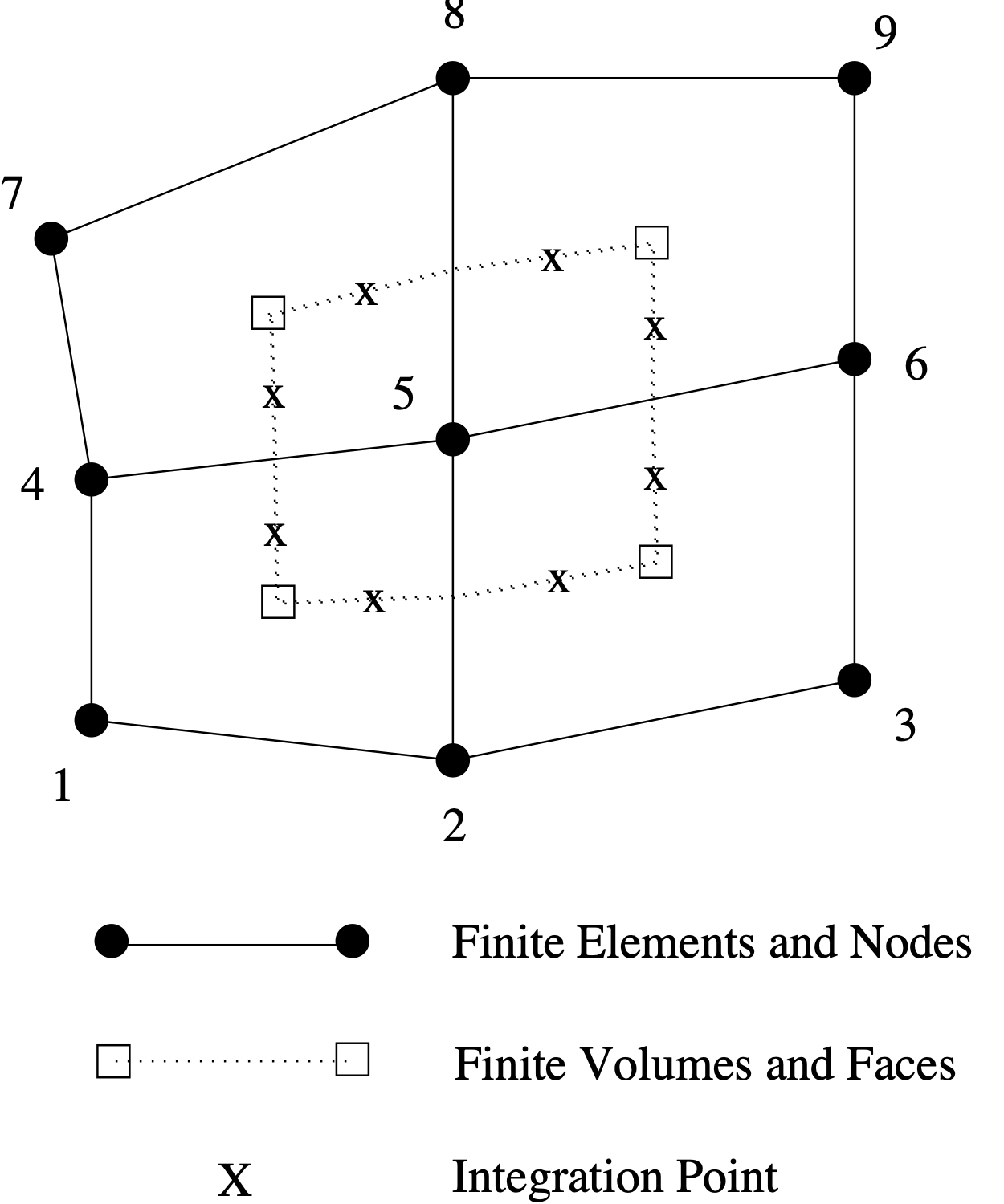
Fig. 3.17 Control Volume is Centered about Finite-Element Node

3.10.1. Integral Form

We begin with the transient weak description (or equivalently the stationary description). As is discussed in [31], the test function is chosen to be a Heaviside function – unity within the control volume and zero outside of it. The gradient of this test function is zero everywhere but the boundaries of the control volume, where it is given by a negative Dirac delta function. This implies that

$- \int_{\Omega} \nabla w \cdot \f = \sum_{e} \int_{\Gamma_e} \f \cdot \vector{d\Gamma_e} \, \text{ ,}$

and the classic finite volume form of the general conservation equation is recovered

(3.190) $\sum_{e} \int_{\Omega_e} \left( \frac{\partial \symSlnVar}{\partial t} - \symSlnVar_\Vol \right) d \Omega_e + \sum_{e} \int_{\Gamma_e} \left( \v \symSlnVar - \f \right) \cdot \vector{d\Gamma_e} = 0$

Here the summation is over each control volume boundary, $\Gamma_e$ , with outward pointing differential area vector $\vector{d\Gamma_e}$ .

Note

This integral form is more commonly derived by integrating the general conservation equation over the control volume and applying the Gauss Divergence Theorem to the result.

3.10.2. CVFEM Operators

Control volumes (the mesh dual) are constructed about the nodes, as shown in Fig. 3.17. As is discussed in Finite Element Approximation, the finite element basis is used to interpolate quantities from the nodes to the interiors of the elements.

Each element contains a set of subfaces that define subcontrol surfaces (SCS). The subfaces consist of line segments (2-D) or surfaces (3-D). The 2-D segments are connected between the element centroid and the edge centroids. The 3-D surfaces are connected between the element centroid, the element face centroids, and the edge centroids. The fluxes across this surface are integrated over the SCS element and the contribution is added to the two connected control volumes.

Integration points also exist within the subcontrol volume (SCV) centroids. Such integration points are used for volume integrals such as source terms, the mass matrix, and gradients as needed. These quantities are similarly numerically integrated over the SCV element.

For transient problems, the time variation of the nodal values is treated in the same way as the Galerkin FEM approach.