3.1. Domain Definition
To fix the notation, consider Fig. 3.1, which is a schematic representation of a
typical problem. The entire domain is represented by
 , which, for example, lies in three-dimensional coordinate space,
with spatial coordinates
, which, for example, lies in three-dimensional coordinate space,
with spatial coordinates  . In this particular
case, consists of two separate subdomains,
. In this particular
case, consists of two separate subdomains,
 . These subdomains may consist of
different materials. The entire boundary of is indicated
by
. These subdomains may consist of
different materials. The entire boundary of is indicated
by  ,
subject to one or more boundary conditions on subsections we denote
with a subscript on
,
subject to one or more boundary conditions on subsections we denote
with a subscript on  .
For example, let
.
For example, let  be that portion of
along which a specified heat flux normal to the
boundary is applied; similarly, let
be that portion of
along which a specified heat flux normal to the
boundary is applied; similarly, let  be subject to an applied temperature; let the surface
 be adiabatic (no heat flux); let
 , be subject to an applied radiation
heat flux; and let
, be subject to an applied radiation
heat flux; and let  be subject to a
convective heat flux, which is modeled by Newton’s law of
cooling. Note that the boundary conditions are of two types:
either the flux or the temperature is specified. Finally, the
interface between
be subject to a
convective heat flux, which is modeled by Newton’s law of
cooling. Note that the boundary conditions are of two types:
either the flux or the temperature is specified. Finally, the
interface between  and
and  is denoted
 . The
interface conditions applied along a boundary such as
are that both the temperature and the
normal component of the heat flux are continuous. Given
appropriate initial conditions, the problem is to determine the
time-evolution of the temperature field.
. The
interface conditions applied along a boundary such as
are that both the temperature and the
normal component of the heat flux are continuous. Given
appropriate initial conditions, the problem is to determine the
time-evolution of the temperature field.
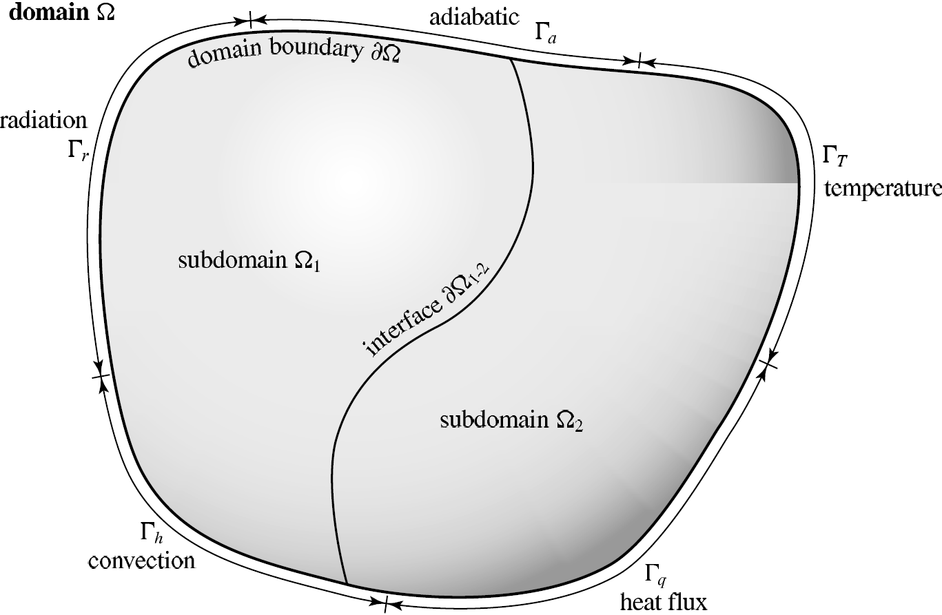
Fig. 3.1 A schematic diagram of the mathematical thermal model, showing the
domain ; the subdomains  and their
interfaces
and their
interfaces  ; and the boundary
conditions on the surface .
; and the boundary
conditions on the surface .
Note that when referencing a generic volume or surface,  and
and
 will be used respectively.