3.9. Finite Element Approximation
In Discretization, we discretized the governing equations in space using Galerkin’s method. In this chapter, we discuss two important, unresolved issues. The first issue is the method for constructing the basis functions  , which appear in the weak statements given by the stationary weak description and the transient weak description. The second issue is the calculation of the associated integrals over the domain and its boundary. The finite element method solves both of these issues, and is concisely described by Becker, et al [22]:
The finite element method provides a general and systematic technique for constructing basis functions for Galerkin approximations of boundary value problems. The main idea is that the basis functions […] can be defined piecewise over subregions of the domain called finite elements and that over any subdomain the [basis functions] can be chosen to be very simple functions such as polynomials of low degree.
If the finite elements are also chosen to have convenient shapes (like triangles and quadrilaterals) for calculating integrals, then the integration over the entire domain is also facilitated.
To elaborate, consider Fig. 3.10, which shows a one-dimensional domain partitioned into four finite elements. In Fig. 3.11, the global, piecewise linear basis function for node i,  , is shown as the standard hat function. This function has a value of unity at node i and zero in elements not connected to node i. The finite element approach to constructing is shown in Fig. 3.11. On each element, two linear functions
  are defined,
  ,
,  . If we add
  from the left element to
  from the right element, then we see that the global basis function is constructed.
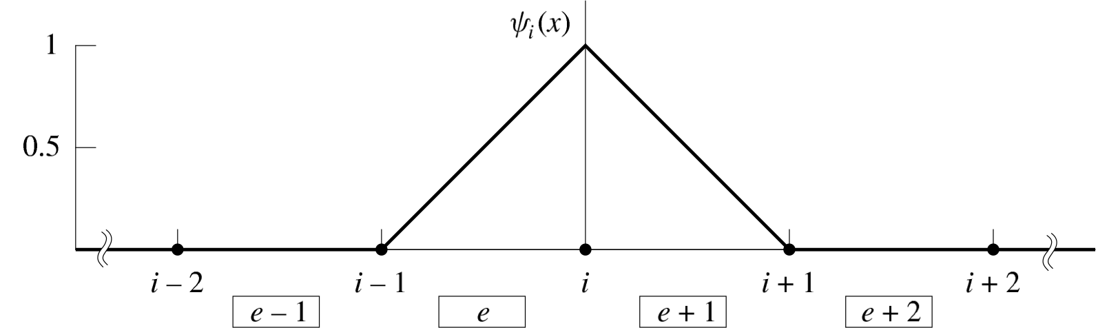
Fig. 3.10 A linear finite element global basis function at a node is formed from the nodal shape functions of two neighboring elements. The global basis function for node  has support over the two elements
  and
and  that share the node, and takes on the value of zero everywhere else.
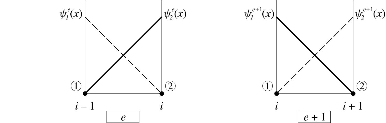
Fig. 3.11 The associated element shape functions,  (on local node 2 of element ), and
  (on local node 1 of element ), are combined to define the global basis function for node .
Locally, the element’s shape functions can be used to interpolate values defined at the nodes to arbitrary location within the element. Specifically, for some quantity  defined at the
  (local) nodes of the element , the value of within the element is

Now, consider the global stiffness matrix  , with row and column
  , defined in the previous section. We now rewrite this integral as the sum over each finite element, namely
(3.168)
In (3.168), the global basis function is nonzero only on those elements which support node . Hence we can consider the contributions to the global stiffness matrix from element , and define
(3.169)
There is a subtle difference in the interpretation of the indices in (3.168) as opposed to (3.169). In (3.168), the indices and are global, and span all nodes in the finite element mesh. In (3.169), the indices and are local, and only span the number of element shape functions. Aria calculates the element stiffness matrix contributions defined in (3.169) and assembles the results into the correct locations in the global stiffness matrix using a mapping from the local node numbers of a given element to the associated global node numbers. In fact, each of the integrals in the weak statements derived in Discretization involves a basis function and is calculated in the same way.
In the following section, Element Integration, we discuss how the integrals are computed on a master element. Next, in Linear Master Elements, we discuss the master element interpolation functions for the elements used in Aria.
3.9.1. Element Integration
Element integrals of the form given by (3.169) are defined on the element coordinates in physical space. When calculating these quantities numerically, it is convenient to transform these integrals from physical space to a reference element, also called a master element, in parametric space. This transformation is performed locally, for each finite element in the mesh. In this section we discuss the details of this process for two-dimensional physical space in Cartesian coordinates. The approach is completely general, and extensible to three-dimensional space and other coordinate systems. This situation is illustrated in Fig. 3.12, showing such a transformation from the quadrilateral element, which spans the region ![[-1,1]\times[-1,1]](data:image/svg+xml;base64,PD94bWwgdmVyc2lvbj0nMS4wJyBlbmNvZGluZz0nVVRGLTgnPz4KPCEtLSBUaGlzIGZpbGUgd2FzIGdlbmVyYXRlZCBieSBkdmlzdmdtIDMuMC4zIC0tPgo8c3ZnIHZlcnNpb249JzEuMScgeG1sbnM9J2h0dHA6Ly93d3cudzMub3JnLzIwMDAvc3ZnJyB4bWxuczp4bGluaz0naHR0cDovL3d3dy53My5vcmcvMTk5OS94bGluaycgd2lkdGg9JzkzLjQ2ODQzNnB0JyBoZWlnaHQ9JzEzLjk0NzY5NnB0JyB2aWV3Qm94PScwIC0xMC40NjA3NzIgOTMuNDY4NDM2IDEzLjk0NzY5Nic+CjxkZWZzPgo8cGF0aCBpZD0nZzEtNTknIGQ9J00yLjcxOTgwMSAuMDU1NzkxQzIuNzE5ODAxLS43NTMxNzYgMi40NTQ3OTUtMS4zNTI5MjcgMS44ODI5MzktMS4zNTI5MjdDMS40MzY2MTMtMS4zNTI5MjcgMS4yMTM0NS0uOTkwMjg2IDEuMjEzNDUtLjY4MzQzN1MxLjQyMjY2NSAwIDEuODk2ODg3IDBDMi4wNzgyMDcgMCAyLjIzMTYzMS0uMDU1NzkxIDIuMzU3MTYxLS4xODEzMkMyLjM4NTA1Ni0uMjA5MjE1IDIuMzk5MDA0LS4yMDkyMTUgMi40MTI5NTEtLjIwOTIxNUMyLjQ0MDg0Ny0uMjA5MjE1IDIuNDQwODQ3LS4wMTM5NDggMi40NDA4NDcgLjA1NTc5MUMyLjQ0MDg0NyAuNTE2MDY1IDIuMzU3MTYxIDEuNDIyNjY1IDEuNTQ4MTk0IDIuMzI5MjY1QzEuMzk0NzcgMi40OTY2MzggMS4zOTQ3NyAyLjUyNDUzMyAxLjM5NDc3IDIuNTUyNDI4QzEuMzk0NzcgMi42MjIxNjcgMS40NjQ1MDggMi42OTE5MDUgMS41MzQyNDcgMi42OTE5MDVDMS42NDU4MjggMi42OTE5MDUgMi43MTk4MDEgMS42NTk3NzYgMi43MTk4MDEgLjA1NTc5MVonLz4KPHBhdGggaWQ9J2cyLTQ5JyBkPSdNNC4wMTY5MzYtOC45NDA0NzNDNC4wMTY5MzYtOS4yNjEyNyA0LjAxNjkzNi05LjI3NTIxOCAzLjczNzk4My05LjI3NTIxOEMzLjQwMzIzOC04Ljg5ODYzIDIuNzA1ODUzLTguMzgyNTY1IDEuMjY5MjQtOC4zODI1NjVWLTcuOTc4MDgyQzEuNTkwMDM3LTcuOTc4MDgyIDIuMjg3NDIyLTcuOTc4MDgyIDMuMDU0NTQ1LTguMzQwNzIyVi0xLjA3Mzk3M0MzLjA1NDU0NS0uNTcxODU2IDMuMDEyNzAyLS40MDQ0ODMgMS43ODUzMDUtLjQwNDQ4M0gxLjM1MjkyN1YwQzEuNzI5NTE0LS4wMjc4OTUgMy4wODI0NDEtLjAyNzg5NSAzLjU0MjcxNS0uMDI3ODk1UzUuMzQxOTY4LS4wMjc4OTUgNS43MTg1NTUgMFYtLjQwNDQ4M0g1LjI4NjE3N0M0LjA1ODc4LS40MDQ0ODMgNC4wMTY5MzYtLjU3MTg1NiA0LjAxNjkzNi0xLjA3Mzk3M1YtOC45NDA0NzNaJy8+CjxwYXRoIGlkPSdnMi05MScgZD0nTTMuNDg2OTI0IDMuNDg2OTI0VjIuOTcwODU5SDIuMTMzOTk4Vi05Ljk0NDcwN0gzLjQ4NjkyNFYtMTAuNDYwNzcySDEuNjE3OTMzVjMuNDg2OTI0SDMuNDg2OTI0WicvPgo8cGF0aCBpZD0nZzItOTMnIGQ9J00yLjE2MTg5My0xMC40NjA3NzJILjI5MjkwMlYtOS45NDQ3MDdIMS42NDU4MjhWMi45NzA4NTlILjI5MjkwMlYzLjQ4NjkyNEgyLjE2MTg5M1YtMTAuNDYwNzcyWicvPgo8cGF0aCBpZD0nZzAtMCcgZD0nTTkuMTkxNTMyLTMuMjA3OTdDOS40Mjg2NDMtMy4yMDc5NyA5LjY3OTcwMS0zLjIwNzk3IDkuNjc5NzAxLTMuNDg2OTI0UzkuNDI4NjQzLTMuNzY1ODc4IDkuMTkxNTMyLTMuNzY1ODc4SDEuNjQ1ODI4QzEuNDA4NzE3LTMuNzY1ODc4IDEuMTU3NjU5LTMuNzY1ODc4IDEuMTU3NjU5LTMuNDg2OTI0UzEuNDA4NzE3LTMuMjA3OTcgMS42NDU4MjgtMy4yMDc5N0g5LjE5MTUzMlonLz4KPHBhdGggaWQ9J2cwLTInIGQ9J001LjQyNTY1NC0zLjg3NzQ2TDIuNjM2MTE1LTYuNjUzMDUxQzIuNDY4NzQyLTYuODIwNDIzIDIuNDQwODQ3LTYuODQ4MzE5IDIuMzI5MjY1LTYuODQ4MzE5QzIuMTg5Nzg4LTYuODQ4MzE5IDIuMDUwMzExLTYuNzIyNzkgMi4wNTAzMTEtNi41NjkzNjVDMi4wNTAzMTEtNi40NzE3MzEgMi4wNzgyMDctNi40NDM4MzYgMi4yMzE2MzEtNi4yOTA0MTFMNS4wMjExNzEtMy40ODY5MjRMMi4yMzE2MzEtLjY4MzQzN0MyLjA3ODIwNy0uNTMwMDEyIDIuMDUwMzExLS41MDIxMTcgMi4wNTAzMTEtLjQwNDQ4M0MyLjA1MDMxMS0uMjUxMDU5IDIuMTg5Nzg4LS4xMjU1MjkgMi4zMjkyNjUtLjEyNTUyOUMyLjQ0MDg0Ny0uMTI1NTI5IDIuNDY4NzQyLS4xNTM0MjUgMi42MzYxMTUtLjMyMDc5N0w1LjQxMTcwNi0zLjA5NjM4OUw4LjI5ODg3OS0uMjA5MjE1QzguMzI2Nzc1LS4xOTUyNjggOC40MjQ0MDgtLjEyNTUyOSA4LjUwODA5NS0uMTI1NTI5QzguNjc1NDY3LS4xMjU1MjkgOC43ODcwNDktLjI1MTA1OSA4Ljc4NzA0OS0uNDA0NDgzQzguNzg3MDQ5LS40MzIzNzkgOC43ODcwNDktLjQ4ODE2OSA4Ljc0NTIwNS0uNTU3OTA4QzguNzMxMjU4LS41ODU4MDMgNi41MTM1NzQtMi43NzU1OTIgNS44MTYxODktMy40ODY5MjRMOC4zNjg2MTgtNi4wMzkzNTJDOC40MzgzNTYtNi4xMjMwMzkgOC42NDc1NzItNi4zMDQzNTkgOC43MTczMS02LjM4ODA0NUM4LjczMTI1OC02LjQxNTk0IDguNzg3MDQ5LTYuNDcxNzMxIDguNzg3MDQ5LTYuNTY5MzY1QzguNzg3MDQ5LTYuNzIyNzkgOC42NzU0NjctNi44NDgzMTkgOC41MDgwOTUtNi44NDgzMTlDOC4zOTY1MTMtNi44NDgzMTkgOC4zNDA3MjItNi43OTI1MjggOC4xODcyOTgtNi42MzkxMDNMNS40MjU2NTQtMy44Nzc0NlonLz4KPC9kZWZzPgo8ZyBpZD0ncGFnZTEnPgo8dXNlIHg9JzAnIHk9JzAnIHhsaW5rOmhyZWY9JyNnMi05MScvPgo8dXNlIHg9JzMuNzkzNjA1JyB5PScwJyB4bGluazpocmVmPScjZzAtMCcvPgo8dXNlIHg9JzE0LjY0MTg1MScgeT0nMCcgeGxpbms6aHJlZj0nI2cyLTQ5Jy8+Cjx1c2UgeD0nMjEuNDcwMzQnIHk9JzAnIHhsaW5rOmhyZWY9JyNnMS01OScvPgo8dXNlIHg9JzI3LjU4ODU0MScgeT0nMCcgeGxpbms6aHJlZj0nI2cyLTQ5Jy8+Cjx1c2UgeD0nMzQuNDE3MDI5JyB5PScwJyB4bGluazpocmVmPScjZzItOTMnLz4KPHVzZSB4PSc0MS4zMTAwOTUnIHk9JzAnIHhsaW5rOmhyZWY9JyNnMC0yJy8+Cjx1c2UgeD0nNTUuMjU3ODAyJyB5PScwJyB4bGluazpocmVmPScjZzItOTEnLz4KPHVzZSB4PSc1OS4wNTE0MDcnIHk9JzAnIHhsaW5rOmhyZWY9JyNnMC0wJy8+Cjx1c2UgeD0nNjkuODk5NjU0JyB5PScwJyB4bGluazpocmVmPScjZzItNDknLz4KPHVzZSB4PSc3Ni43MjgxNDInIHk9JzAnIHhsaW5rOmhyZWY9JyNnMS01OScvPgo8dXNlIHg9JzgyLjg0NjM0MycgeT0nMCcgeGxpbms6aHJlZj0nI2cyLTQ5Jy8+Cjx1c2UgeD0nODkuNjc0ODMyJyB5PScwJyB4bGluazpocmVmPScjZzItOTMnLz4KPC9nPgo8L3N2Zz4KPCEtLSBERVBUSD01IC0tPg==) , in parametric coordinates
, in parametric coordinates  to an arbitrary region in physical coordinates
  .
.
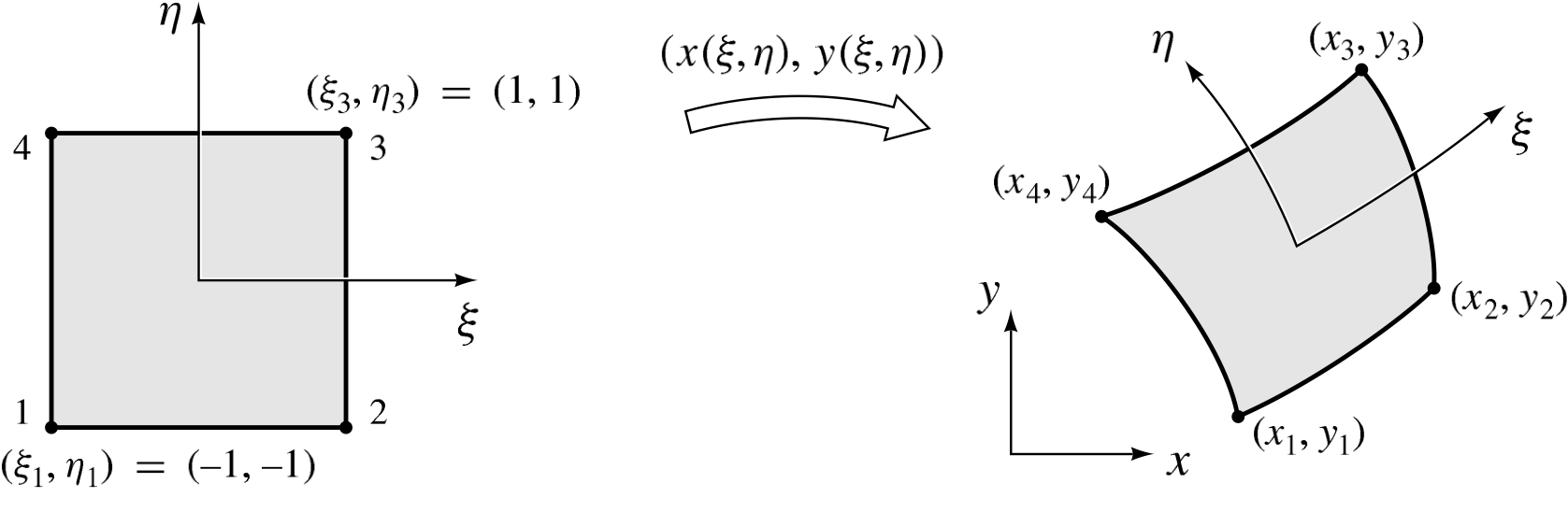
Fig. 3.12 Mapping from the master element to physical coordinates: The quadrilateral master element in on the region is mapped to its image in physical coordinates .
Returning to
(3.169), given some function  , we wish to
calculate the integral
, we wish to
calculate the integral
(3.170)
on the master element in space. The change of
variables theorem [28] from vector calculus states that
(3.170) is equivalent to
(3.171)
where  is the master element and
  is the
determinant of the non-singular Jacobian matrix of the transformation
is the
determinant of the non-singular Jacobian matrix of the transformation
(3.172)
Recall the Jacobian matrix of (3.172)
(3.173)![\mathbf{J} = %
\begin{pmatrix}
\dfrac{\partial x}{\partial \xi} & \dfrac{\partial x}{\partial \eta}\\[12pt] %
\dfrac{\partial y}{\partial \xi} & \dfrac{\partial y}{\partial \eta} %
\end{pmatrix}](data:image/svg+xml;base64,PD94bWwgdmVyc2lvbj0nMS4wJyBlbmNvZGluZz0nVVRGLTgnPz4KPCEtLSBUaGlzIGZpbGUgd2FzIGdlbmVyYXRlZCBieSBkdmlzdmdtIDMuMC4zIC0tPgo8c3ZnIHZlcnNpb249JzEuMScgeG1sbnM9J2h0dHA6Ly93d3cudzMub3JnLzIwMDAvc3ZnJyB4bWxuczp4bGluaz0naHR0cDovL3d3dy53My5vcmcvMTk5OS94bGluaycgd2lkdGg9Jzk3LjA4NTczMXB0JyBoZWlnaHQ9JzY3LjU1ODgzcHQnIHZpZXdCb3g9JzE0NS43Mjg2MTggLTY3LjU1ODgzMiA5Ny4wODU3MzEgNjcuNTU4ODMnPgo8ZGVmcz4KPHBhdGggaWQ9J2cxLTQ4JyBkPSdNNS4yMTY0MzggMjQuNjg3NDIyQzUuNTIzMjg4IDI0LjY4NzQyMiA1LjYwNjk3NCAyNC42ODc0MjIgNS42MDY5NzQgMjQuNDkyMTU0QzUuNjM0ODY5IDE0LjcxNDgxOSA2Ljc2NDYzMyA2LjU5NzI2IDExLjY0NjMyNi0uMjIzMTYzQzExLjc0Mzk2LS4zNDg2OTIgMTEuNzQzOTYtLjM3NjU4OCAxMS43NDM5Ni0uNDA0NDgzQzExLjc0Mzk2LS41NDM5NiAxMS42NDYzMjYtLjU0Mzk2IDExLjQyMzE2My0uNTQzOTZTMTEuMTcyMTA1LS41NDM5NiAxMS4xNDQyMDktLjUxNjA2NUMxMS4wODg0MTgtLjQ3NDIyMiA5LjMxNzA2MSAxLjU2MjE0MiA3LjkwODM0NCA0LjM2NTYyOUM2LjA2NzI0OCA4LjA0NzgyMSA0LjkwOTU4OSAxMi4yNzM5NzMgNC4zOTM1MjQgMTcuMzUwOTM0QzQuMzUxNjgxIDE3Ljc4MzMxMyA0LjA1ODc4IDIwLjY4NDQzMyA0LjA1ODc4IDIzLjk5MDAzN1YyNC41MzM5OThDNC4wNzI3MjcgMjQuNjg3NDIyIDQuMTU2NDEzIDI0LjY4NzQyMiA0LjQ0OTMxNSAyNC42ODc0MjJINS4yMTY0MzhaJy8+CjxwYXRoIGlkPSdnMS00OScgZD0nTTguMTMxNTA3IDIzLjk5MDAzN0M4LjEzMTUwNyAxNS40Njc5OTUgNi42MTEyMDggMTAuNDc0NzIgNi4xNzg4MjkgOS4wNjYwMDJDNS4yMzAzODYgNS45Njk2MTQgMy42ODIxOTIgMi43MDU4NTMgMS4zNTI5MjctLjE2NzM3MkMxLjE0MzcxMS0uNDE4NDMxIDEuMDg3OTItLjQ4ODE2OSAxLjAzMjEzLS41MTYwNjVDMS4wMDQyMzQtLjUzMDAxMiAuOTkwMjg2LS41NDM5NiAuNzY3MTIzLS41NDM5NkMuNTU3OTA4LS41NDM5NiAuNDQ2MzI2LS41NDM5NiAuNDQ2MzI2LS40MDQ0ODNDLjQ0NjMyNi0uMzc2NTg4IC40NDYzMjYtLjM0ODY5MiAuNjI3NjQ2LS4wOTc2MzRDNS40ODE0NDUgNi42ODA5NDYgNi41NjkzNjUgMTUuMDQ5NTY0IDYuNTgzMzEzIDI0LjQ5MjE1NEM2LjU4MzMxMyAyNC42ODc0MjIgNi42NjY5OTkgMjQuNjg3NDIyIDYuOTczODQ4IDI0LjY4NzQyMkg3Ljc0MDk3MUM4LjAzMzg3MyAyNC42ODc0MjIgOC4xMTc1NTkgMjQuNjg3NDIyIDguMTMxNTA3IDI0LjUzMzk5OFYyMy45OTAwMzdaJy8+CjxwYXRoIGlkPSdnMS02NCcgZD0nTTQuNDQ5MzE1LS42OTczODVDNC4xNTY0MTMtLjY5NzM4NSA0LjA3MjcyNy0uNjk3Mzg1IDQuMDU4NzgtLjU0Mzk2VjBDNC4wNTg3OCA4LjUyMjA0MiA1LjU3OTA3OCAxMy41MTUzMTggNi4wMTE0NTcgMTQuOTI0MDM1QzYuOTU5OSAxOC4wMjA0MjMgOC41MDgwOTUgMjEuMjg0MTg0IDEwLjgzNzM2IDI0LjE1NzQxQzExLjA0NjU3NSAyNC40MDg0NjggMTEuMTAyMzY2IDI0LjQ3ODIwNyAxMS4xNTgxNTcgMjQuNTA2MTAyQzExLjE4NjA1MiAyNC41MjAwNSAxMS4yIDI0LjUzMzk5OCAxMS40MjMxNjMgMjQuNTMzOTk4UzExLjc0Mzk2IDI0LjUzMzk5OCAxMS43NDM5NiAyNC4zOTQ1MjFDMTEuNzQzOTYgMjQuMzY2NjI1IDExLjc0Mzk2IDI0LjMzODczIDExLjY2MDI3NCAyNC4yMTMyQzcuMDE1NjkxIDE3Ljc2OTM2NSA1LjYyMDkyMiAxMC4wMTQ0NDYgNS42MDY5NzQtLjUwMjExN0M1LjYwNjk3NC0uNjk3Mzg1IDUuNTIzMjg4LS42OTczODUgNS4yMTY0MzgtLjY5NzM4NUg0LjQ0OTMxNVonLz4KPHBhdGggaWQ9J2cxLTY1JyBkPSdNOC4xMzE1MDctLjU0Mzk2QzguMTE3NTU5LS42OTczODUgOC4wMzM4NzMtLjY5NzM4NSA3Ljc0MDk3MS0uNjk3Mzg1SDYuOTczODQ4QzYuNjY2OTk5LS42OTczODUgNi41ODMzMTMtLjY5NzM4NSA2LjU4MzMxMy0uNTAyMTE3QzYuNTgzMzEzIC45MzQ0OTYgNi41NjkzNjUgNC4yNTQwNDcgNi4yMDY3MjUgNy43MjcwMjRDNS40NTM1NDkgMTQuOTM3OTgzIDMuNTk4NTA2IDE5LjkzMTI1OCAuNTQzOTYgMjQuMjEzMkMuNDQ2MzI2IDI0LjMzODczIC40NDYzMjYgMjQuMzY2NjI1IC40NDYzMjYgMjQuMzk0NTIxQy40NDYzMjYgMjQuNTMzOTk4IC41NTc5MDggMjQuNTMzOTk4IC43NjcxMjMgMjQuNTMzOTk4Qy45OTAyODYgMjQuNTMzOTk4IDEuMDE4MTgyIDI0LjUzMzk5OCAxLjA0NjA3NyAyNC41MDYxMDJDMS4xMDE4NjggMjQuNDY0MjU5IDIuODczMjI1IDIyLjQyNzg5NSA0LjI4MTk0MyAxOS42MjQ0MDhDNi4xMjMwMzkgMTUuOTQyMjE3IDcuMjgwNjk3IDExLjcxNjA2NSA3Ljc5Njc2MiA2LjYzOTEwM0M3LjgzODYwNSA2LjIwNjcyNSA4LjEzMTUwNyAzLjMwNTYwNCA4LjEzMTUwNyAwVi0uNTQzOTZaJy8+CjxwYXRoIGlkPSdnMS02NicgZD0nTTUuNjA2OTc0IC4yMzcxMTFDNS42MDY5NzQtLjEyNTUyOSA1LjU5MzAyNi0uMTM5NDc3IDUuMjE2NDM4LS4xMzk0NzdINC40NDkzMTVDNC4wNzI3MjctLjEzOTQ3NyA0LjA1ODc4LS4xMjU1MjkgNC4wNTg3OCAuMjM3MTExVjguMTMxNTA3QzQuMDU4NzggOC40OTQxNDcgNC4wNzI3MjcgOC41MDgwOTUgNC40NDkzMTUgOC41MDgwOTVINS4yMTY0MzhDNS41OTMwMjYgOC41MDgwOTUgNS42MDY5NzQgOC40OTQxNDcgNS42MDY5NzQgOC4xMzE1MDdWLjIzNzExMVonLz4KPHBhdGggaWQ9J2cxLTY3JyBkPSdNOC4xMzE1MDcgLjIzNzExMUM4LjEzMTUwNy0uMTI1NTI5IDguMTE3NTU5LS4xMzk0NzcgNy43NDA5NzEtLjEzOTQ3N0g2Ljk3Mzg0OEM2LjU5NzI2LS4xMzk0NzcgNi41ODMzMTMtLjEyNTUyOSA2LjU4MzMxMyAuMjM3MTExVjguMTMxNTA3QzYuNTgzMzEzIDguNDk0MTQ3IDYuNTk3MjYgOC41MDgwOTUgNi45NzM4NDggOC41MDgwOTVINy43NDA5NzFDOC4xMTc1NTkgOC41MDgwOTUgOC4xMzE1MDcgOC40OTQxNDcgOC4xMzE1MDcgOC4xMzE1MDdWLjIzNzExMVonLz4KPHBhdGggaWQ9J2cwLTc0JyBkPSdNNi4wODExOTYtOC45NjgzNjlINy4xOTcwMTFWLTkuNTY4MTJDNi44NDgzMTktOS41NDAyMjQgNS40MTE3MDYtOS41NDAyMjQgNC45NjUzOC05LjU0MDIyNEM0LjI0MDEtOS41NDAyMjQgMy4wNjg0OTMtOS41NDAyMjQgMi4zODUwNTYtOS41NjgxMlYtOC45NjgzNjlINC4zMDk4MzhWLTIuMDc4MjA3QzQuMzA5ODM4LS43NjcxMjMgMy42NjgyNDQtLjI5MjkwMiAyLjk0Mjk2NC0uMjkyOTAyQzIuODQ1MzMtLjI5MjkwMiAyLjIwMzczNi0uMjkyOTAyIDEuNjU5Nzc2LS42NDE1OTRDMi4xNjE4OTMtLjc2NzEyMyAyLjM5OTAwNC0xLjE3MTYwNiAyLjM5OTAwNC0xLjU5MDAzN0MyLjM5OTAwNC0yLjI3MzQ3NCAxLjg1NTA0NC0yLjU4MDMyNCAxLjQyMjY2NS0yLjU4MDMyNEMuOTIwNTQ4LTIuNTgwMzI0IC40MzIzNzktMi4yMzE2MzEgLjQzMjM3OS0xLjU5MDAzN0MuNDMyMzc5LS41NDM5NiAxLjUwNjM1MSAuMTY3MzcyIDMuMDEyNzAyIC4xNjczNzJDNC43OTgwMDcgLjE2NzM3MiA2LjA4MTE5Ni0uNjQxNTk0IDYuMDgxMTk2LTIuMDc4MjA3Vi04Ljk2ODM2OVonLz4KPHBhdGggaWQ9J2cyLTE3JyBkPSdNNi42MjUxNTYtMy44NjM1MTJDNi42OTQ4OTQtNC4xNDI0NjYgNi43MzY3MzctNC4zMDk4MzggNi43MzY3MzctNC42ODY0MjZDNi43MzY3MzctNS41MjMyODggNi4yNDg1NjgtNi4xNTA5MzQgNS4xODg1NDMtNi4xNTA5MzRDMy45NDcxOTgtNi4xNTA5MzQgMy4yOTE2NTYtNS4yNzIyMjkgMy4wNDA1OTgtNC45MjM1MzdDMi45OTg3NTUtNS43MTg1NTUgMi40MjY4OTktNi4xNTA5MzQgMS44MTMyLTYuMTUwOTM0QzEuNDA4NzE3LTYuMTUwOTM0IDEuMDg3OTItNS45NTU2NjYgLjgyMjkxNC01LjQyNTY1NEMuNTcxODU2LTQuOTIzNTM3IC4zNzY1ODgtNC4wNzI3MjcgLjM3NjU4OC00LjAxNjkzNlMuNDMyMzc5LTMuODkxNDA3IC41MzAwMTItMy44OTE0MDdDLjY0MTU5NC0zLjg5MTQwNyAuNjU1NTQyLTMuOTA1MzU1IC43MzkyMjgtNC4yMjYxNTJDLjk0ODQ0My01LjA0OTA2NiAxLjIxMzQ1LTUuODcxOTggMS43NzEzNTctNS44NzE5OEMyLjA5MjE1NC01Ljg3MTk4IDIuMjAzNzM2LTUuNjQ4ODE3IDIuMjAzNzM2LTUuMjMwMzg2QzIuMjAzNzM2LTQuOTIzNTM3IDIuMDY0MjU5LTQuMzc5NTc3IDEuOTY2NjI1LTMuOTQ3MTk4TDEuNTc2MDktMi40NDA4NDdDMS41MjAyOTktMi4xNzU4NDEgMS4zNjY4NzQtMS41NDgxOTQgMS4yOTcxMzYtMS4yOTcxMzZDMS4xOTk1MDItLjkzNDQ5NiAxLjA0NjA3Ny0uMjc4OTU0IDEuMDQ2MDc3LS4yMDkyMTVDMS4wNDYwNzctLjAxMzk0OCAxLjE5OTUwMiAuMTM5NDc3IDEuNDA4NzE3IC4xMzk0NzdDMS41NzYwOSAuMTM5NDc3IDEuNzcxMzU3IC4wNTU3OTEgMS44ODI5MzktLjE1MzQyNUMxLjkxMDgzNC0uMjIzMTYzIDIuMDM2MzY0LS43MTEzMzMgMi4xMDYxMDItLjk5MDI4NkwyLjQxMjk1MS0yLjI0NTU3OUwyLjg3MzIyNS00LjA4NjY3NUMyLjkwMTEyMS00LjE3MDM2MSAzLjI0OTgxMy00Ljg2Nzc0NiAzLjc2NTg3OC01LjMxNDA3MkM0LjEyODUxOC01LjY0ODgxNyA0LjYwMjc0LTUuODcxOTggNS4xNDY3LTUuODcxOThDNS43MDQ2MDgtNS44NzE5OCA1Ljg5OTg3NS01LjQ1MzU0OSA1Ljg5OTg3NS00Ljg5NTY0MUM1Ljg5OTg3NS00LjQ5MTE1OCA1Ljg0NDA4NS00LjI2Nzk5NSA1Ljc3NDM0Ni00LjAwMjk4OUw0LjE1NjQxMyAyLjQxMjk1MUM0LjE0MjQ2NiAyLjQ4MjY5IDQuMTE0NTcgMi41NjYzNzYgNC4xMTQ1NyAyLjY1MDA2MkM0LjExNDU3IDIuODU5Mjc4IDQuMjgxOTQzIDIuOTk4NzU1IDQuNDkxMTU4IDIuOTk4NzU1QzQuNjE2Njg3IDIuOTk4NzU1IDQuOTA5NTg5IDIuOTQyOTY0IDUuMDIxMTcxIDIuNTI0NTMzTDYuNjI1MTU2LTMuODYzNTEyWicvPgo8cGF0aCBpZD0nZzItMjQnIGQ9J00zLjY0MDM0OSAuMDY5NzM4TDIuMTc1ODQxLS41MTYwNjVDMS44MTMyLS42NTU1NDIgLjk3NjMzOS0uOTkwMjg2IC45NzYzMzktMS44MjcxNDhDLjk3NjMzOS0zLjAyNjY1IDIuNDQwODQ3LTQuMjQwMSAyLjczMzc0OC00LjI0MDFDMi43NjE2NDQtNC4yNDAxIDIuODg3MTczLTQuMjEyMjA0IDIuOTI5MDE2LTQuMTk4MjU3QzMuMzA1NjA0LTQuMDg2Njc1IDMuNjY4MjQ0LTQuMDg2Njc1IDMuOTE5MzAzLTQuMDg2Njc1QzQuMzUxNjgxLTQuMDg2Njc1IDUuMTc0NTk1LTQuMDg2Njc1IDUuMTc0NTk1LTQuNDkxMTU4QzUuMTc0NTk1LTQuNzk4MDA3IDQuNjcyNDc4LTQuODM5ODUxIDQuMDcyNzI3LTQuODM5ODUxQzMuNzkzNzczLTQuODM5ODUxIDMuNDE3MTg2LTQuODM5ODUxIDIuOTE1MDY4LTQuNjcyNDc4QzIuNTgwMzI0LTQuOTUxNDMyIDIuNDQwODQ3LTUuMzk3NzU4IDIuNDQwODQ3LTUuODE2MTg5QzIuNDQwODQ3LTYuNTgzMzEzIDIuOTQyOTY0LTcuNjcxMjMzIDQuMDQ0ODMyLTguMTg3Mjk4QzQuMjk1ODktNy44OTQzOTYgNC42MzA2MzUtNy44OTQzOTYgNC45MjM1MzctNy44OTQzOTZDNS4yNzIyMjktNy44OTQzOTYgNi4xMjMwMzktNy44OTQzOTYgNi4xMjMwMzktOC4yOTg4NzlDNi4xMjMwMzktOC42NDc1NzIgNS40NTM1NDktOC42NDc1NzIgNS4wMDcyMjMtOC42NDc1NzJDNC43MjgyNjktOC42NDc1NzIgNC41MTkwNTQtOC42NDc1NzIgNC4xMjg1MTgtOC41Nzc4MzNDNC4wNTg3OC04Ljc0NTIwNSA0LjA0NDgzMi04Ljc3MzEwMSA0LjA0NDgzMi05LjA3OTk1QzQuMDQ0ODMyLTkuMzMxMDA5IDQuMTAwNjIzLTkuNTI2Mjc2IDQuMTAwNjIzLTkuNTY4MTJDNC4xMDA2MjMtOS42NTE4MDYgNC4wMzA4ODQtOS43MDc1OTcgMy45NjExNDYtOS43MDc1OTdDMy43Mzc5ODMtOS43MDc1OTcgMy43Mzc5ODMtOS4xOTE1MzIgMy43Mzc5ODMtOS4wNzk5NUMzLjczNzk4My04Ljg4NDY4MiAzLjc1MTkzLTguNjg5NDE1IDMuODM1NjE2LTguNTA4MDk1QzIuMTYxODkzLTguMDE5OTI1IDEuNDIyNjY1LTYuODM0MzcxIDEuNDIyNjY1LTUuOTI3NzcxQzEuNDIyNjY1LTUuMDkwOTA5IDEuOTgwNTczLTQuNjMwNjM1IDIuMzU3MTYxLTQuNDIxNDJDLjkyMDU0OC0zLjY0MDM0OSAuMzA2ODQ5LTIuMjE3Njg0IC4zMDY4NDktMS40NjQ1MDhDLjMwNjg0OS0uMjUxMDU5IDEuNDA4NzE3IC4xODEzMiAxLjkxMDgzNCAuMzkwNTM1TDMuMTY2MTI3IC44OTI2NTNDMy41MTQ4MTkgMS4wMTgxODIgNC4wODY2NzUgMS4yNTUyOTMgNC4xODQzMDkgMS4zMTEwODNDNC4zMjM3ODYgMS40MDg3MTcgNC40MzUzNjcgMS41NzYwOSA0LjQzNTM2NyAxLjc5OTI1M0M0LjQzNTM2NyAyLjA5MjE1NCA0LjIxMjIwNCAyLjU2NjM3NiAzLjcyNDAzNSAyLjU2NjM3NkMzLjUxNDgxOSAyLjU2NjM3NiAzLjA1NDU0NSAyLjUxMDU4NSAyLjU1MjQyOCAyLjEzMzk5OEMyLjQ1NDc5NSAyLjA1MDMxMSAyLjQ0MDg0NyAyLjAzNjM2NCAyLjM4NTA1NiAyLjAzNjM2NEMyLjMxNTMxOCAyLjAzNjM2NCAyLjI0NTU3OSAyLjA5MjE1NCAyLjI0NTU3OSAyLjE3NTg0MUMyLjI0NTU3OSAyLjMyOTI2NSAyLjk3MDg1OSAyLjg0NTMzIDMuNzI0MDM1IDIuODQ1MzNDNC42MTY2ODcgMi44NDUzMyA1LjE2MDY0OCAxLjk4MDU3MyA1LjE2MDY0OCAxLjM4MDgyMkM1LjE2MDY0OCAuOTQ4NDQzIDQuOTIzNTM3IC41OTk3NTEgNC40NzcyMSAuNDA0NDgzTDMuNjQwMzQ5IC4wNjk3MzhaTTQuMzUxNjgxLTguMjk4ODc5QzQuNTg4NzkyLTguMzY4NjE4IDQuODM5ODUxLTguMzY4NjE4IDUuMDIxMTcxLTguMzY4NjE4QzUuNDgxNDQ1LTguMzY4NjE4IDUuNTIzMjg4LTguMzU0NjcgNS44MDIyNDItOC4yODQ5MzJDNS42MzQ4NjktOC4yMTUxOTMgNS41MjMyODgtOC4xNzMzNSA0LjkzNzQ4NC04LjE3MzM1QzQuNjcyNDc4LTguMTczMzUgNC41MDUxMDYtOC4xNzMzNSA0LjM1MTY4MS04LjI5ODg3OVpNMy4yNDk4MTMtNC40NzcyMUMzLjU4NDU1OC00LjU2MDg5NyAzLjg5MTQwNy00LjU2MDg5NyA0LjA1ODc4LTQuNTYwODk3QzQuNTE5MDU0LTQuNTYwODk3IDQuNTQ2OTQ5LTQuNTQ2OTQ5IDQuODUzNzk4LTQuNDc3MjFDNC43MDAzNzQtNC40MDc0NzIgNC41NzQ4NDQtNC4zNjU2MjkgMy45NzUwOTMtNC4zNjU2MjlDMy42NDAzNDktNC4zNjU2MjkgMy41MDA4NzItNC4zNjU2MjkgMy4yNDk4MTMtNC40NzcyMVonLz4KPHBhdGggaWQ9J2cyLTY0JyBkPSdNNi4zMzIyNTQtNC42NTg1MzFDNi4yNDg1NjgtNS40Mzk2MDEgNS43NjAzOTktNi4zNzQwOTcgNC41MDUxMDYtNi4zNzQwOTdDMi41Mzg0ODEtNi4zNzQwOTcgLjUzMDAxMi00LjM3OTU3NyAuNTMwMDEyLTIuMTYxODkzQy41MzAwMTItMS4zMTEwODMgMS4xMTU4MTYgLjI5MjkwMiAzLjAxMjcwMiAuMjkyOTAyQzYuMzA0MzU5IC4yOTI5MDIgNy43MTMwNzYtNC41MDUxMDYgNy43MTMwNzYtNi40MTU5NEM3LjcxMzA3Ni04LjQyNDQwOCA2LjU4MzMxMy05Ljk3MjYwMyA0Ljc5ODAwNy05Ljk3MjYwM0MyLjc3NTU5Mi05Ljk3MjYwMyAyLjE3NTg0MS04LjIwMTI0NSAyLjE3NTg0MS03LjgyNDY1OEMyLjE3NTg0MS03LjY5OTEyOCAyLjI1OTUyNy03LjM5MjI3OSAyLjY1MDA2Mi03LjM5MjI3OUMzLjEzODIzMi03LjM5MjI3OSAzLjM0NzQ0Ny03LjgzODYwNSAzLjM0NzQ0Ny04LjA3NTcxNkMzLjM0NzQ0Ny04LjUwODA5NSAyLjkxNTA2OC04LjUwODA5NSAyLjczMzc0OC04LjUwODA5NUMzLjMwNTYwNC05LjU0MDIyNCA0LjM2NTYyOS05LjYzNzg1OCA0Ljc0MjIxNy05LjYzNzg1OEM1Ljk2OTYxNC05LjYzNzg1OCA2Ljc1MDY4NS04LjY2MTUxOSA2Ljc1MDY4NS03LjA5OTM3N0M2Ljc1MDY4NS02LjIwNjcyNSA2LjQ4NTY3OS01LjE3NDU5NSA2LjM0NjIwMi00LjY1ODUzMUg2LjMzMjI1NFpNMy4wNTQ1NDUtLjA4MzY4NkMxLjc0MzQ2Mi0uMDgzNjg2IDEuNTIwMjk5LTEuMTE1ODE2IDEuNTIwMjk5LTEuNzAxNjE5QzEuNTIwMjk5LTIuMzE1MzE4IDEuOTEwODM0LTMuNzUxOTMgMi4xMjAwNS00LjI2Nzk5NUMyLjMwMTM3LTQuNjg2NDI2IDMuMDk2Mzg5LTYuMDk1MTQzIDQuNTQ2OTQ5LTYuMDk1MTQzQzUuODE2MTg5LTYuMDk1MTQzIDYuMTA5MDkxLTQuOTkzMjc1IDYuMTA5MDkxLTQuMjQwMUM2LjEwOTA5MS0zLjIwNzk3IDUuMjAyNDkxLS4wODM2ODYgMy4wNTQ1NDUtLjA4MzY4NlonLz4KPHBhdGggaWQ9J2cyLTEyMCcgZD0nTTYuNjExMjA4LTUuNjkwNjZDNi4xNjQ4ODItNS42MDY5NzQgNS45OTc1MDktNS4yNzIyMjkgNS45OTc1MDktNS4wMDcyMjNDNS45OTc1MDktNC42NzI0NzggNi4yNjI1MTYtNC41NjA4OTcgNi40NTc3ODMtNC41NjA4OTdDNi44NzYyMTQtNC41NjA4OTcgNy4xNjkxMTYtNC45MjM1MzcgNy4xNjkxMTYtNS4zMDAxMjVDNy4xNjkxMTYtNS44ODU5MjggNi40OTk2MjYtNi4xNTA5MzQgNS45MTM4MjMtNi4xNTA5MzRDNS4wNjMwMTQtNi4xNTA5MzQgNC41ODg3OTItNS4zMTQwNzIgNC40NjMyNjMtNS4wNDkwNjZDNC4xNDI0NjYtNi4wOTUxNDMgMy4yNzc3MDktNi4xNTA5MzQgMy4wMjY2NS02LjE1MDkzNEMxLjYwMzk4NS02LjE1MDkzNCAuODUwODA5LTQuMzIzNzg2IC44NTA4MDktNC4wMTY5MzZDLjg1MDgwOS0zLjk2MTE0NiAuOTA2Ni0zLjg5MTQwNyAxLjAwNDIzNC0zLjg5MTQwN0MxLjExNTgxNi0zLjg5MTQwNyAxLjE0MzcxMS0zLjk3NTA5MyAxLjE3MTYwNi00LjAzMDg4NEMxLjY0NTgyOC01LjU3OTA3OCAyLjU4MDMyNC01Ljg3MTk4IDIuOTg0ODA3LTUuODcxOThDMy42MTI0NTMtNS44NzE5OCAzLjczNzk4My01LjI4NjE3NyAzLjczNzk4My00Ljk1MTQzMkMzLjczNzk4My00LjY0NDU4MyAzLjY1NDI5Ni00LjMyMzc4NiAzLjQ4NjkyNC0zLjY1NDI5NkwzLjAxMjcwMi0xLjc0MzQ2MkMyLjgwMzQ4Ny0uOTA2NiAyLjM5OTAwNC0uMTM5NDc3IDEuNjU5Nzc2LS4xMzk0NzdDMS41OTAwMzctLjEzOTQ3NyAxLjI0MTM0NS0uMTM5NDc3IC45NDg0NDMtLjMyMDc5N0MxLjQ1MDU2LS40MTg0MzEgMS41NjIxNDItLjgzNjg2MiAxLjU2MjE0Mi0xLjAwNDIzNEMxLjU2MjE0Mi0xLjI4MzE4OCAxLjM1MjkyNy0xLjQ1MDU2IDEuMDg3OTItMS40NTA1NkMuNzUzMTc2LTEuNDUwNTYgLjM5MDUzNS0xLjE1NzY1OSAuMzkwNTM1LS43MTEzMzNDLjM5MDUzNS0uMTI1NTI5IDEuMDQ2MDc3IC4xMzk0NzcgMS42NDU4MjggLjEzOTQ3N0MyLjMxNTMxOCAuMTM5NDc3IDIuNzg5NTM5LS4zOTA1MzUgMy4wODI0NDEtLjk2MjM5MUMzLjMwNTYwNC0uMTM5NDc3IDQuMDAyOTg5IC4xMzk0NzcgNC41MTkwNTQgLjEzOTQ3N0M1Ljk0MTcxOSAuMTM5NDc3IDYuNjk0ODk0LTEuNjg3NjcxIDYuNjk0ODk0LTEuOTk0NTIxQzYuNjk0ODk0LTIuMDY0MjU5IDYuNjM5MTAzLTIuMTIwMDUgNi41NTU0MTctMi4xMjAwNUM2LjQyOTg4OC0yLjEyMDA1IDYuNDE1OTQtMi4wNTAzMTEgNi4zNzQwOTctMS45Mzg3M0M1Ljk5NzUwOS0uNzExMzMzIDUuMTg4NTQzLS4xMzk0NzcgNC41NjA4OTctLjEzOTQ3N0M0LjA3MjcyNy0uMTM5NDc3IDMuODA3NzIxLS41MDIxMTcgMy44MDc3MjEtMS4wNzM5NzNDMy44MDc3MjEtMS4zODA4MjIgMy44NjM1MTItMS42MDM5ODUgNC4wODY2NzUtMi41MjQ1MzNMNC41NzQ4NDQtNC40MjE0MkM0Ljc4NDA2LTUuMjU4MjgxIDUuMjU4MjgxLTUuODcxOTggNS44OTk4NzUtNS44NzE5OEM1LjkyNzc3MS01Ljg3MTk4IDYuMzE4MzA2LTUuODcxOTggNi42MTEyMDgtNS42OTA2NlonLz4KPHBhdGggaWQ9J2cyLTEyMScgZD0nTTMuNjY4MjQ0IDEuNTYyMTQyQzMuMjkxNjU2IDIuMDkyMTU0IDIuNzQ3Njk2IDIuNTY2Mzc2IDIuMDY0MjU5IDIuNTY2Mzc2QzEuODk2ODg3IDIuNTY2Mzc2IDEuMjI3Mzk3IDIuNTM4NDgxIDEuMDE4MTgyIDEuODk2ODg3QzEuMDYwMDI1IDEuOTEwODM0IDEuMTI5NzYzIDEuOTEwODM0IDEuMTU3NjU5IDEuOTEwODM0QzEuNTc2MDkgMS45MTA4MzQgMS44NTUwNDQgMS41NDgxOTQgMS44NTUwNDQgMS4yMjczOTdTMS41OTAwMzcgLjc5NTAxOSAxLjM4MDgyMiAuNzk1MDE5QzEuMTU3NjU5IC43OTUwMTkgLjY2OTQ4OSAuOTYyMzkxIC42Njk0ODkgMS42NDU4MjhDLjY2OTQ4OSAyLjM1NzE2MSAxLjI2OTI0IDIuODQ1MzMgMi4wNjQyNTkgMi44NDUzM0MzLjQ1OTAyOSAyLjg0NTMzIDQuODY3NzQ2IDEuNTYyMTQyIDUuMjU4MjgxIC4wMTM5NDhMNi42MjUxNTYtNS40MjU2NTRDNi42MzkxMDMtNS40OTUzOTIgNi42NjY5OTktNS41NzkwNzggNi42NjY5OTktNS42NjI3NjVDNi42NjY5OTktNS44NzE5OCA2LjQ5OTYyNi02LjAxMTQ1NyA2LjI5MDQxMS02LjAxMTQ1N0M2LjE2NDg4Mi02LjAxMTQ1NyA1Ljg3MTk4LTUuOTU1NjY2IDUuNzYwMzk5LTUuNTM3MjM1TDQuNzI4MjY5LTEuNDM2NjEzQzQuNjU4NTMxLTEuMTg1NTU0IDQuNjU4NTMxLTEuMTU3NjU5IDQuNTQ2OTQ5LTEuMDA0MjM0QzQuMjY3OTk1LS42MTM2OTkgMy44MDc3MjEtLjEzOTQ3NyAzLjEzODIzMi0uMTM5NDc3QzIuMzU3MTYxLS4xMzk0NzcgMi4yODc0MjItLjkwNjYgMi4yODc0MjItMS4yODMxODhDMi4yODc0MjItMi4wNzgyMDcgMi42NjQwMS0zLjE1MjE3OSAzLjA0MDU5OC00LjE1NjQxM0MzLjE5NDAyMi00LjU2MDg5NyAzLjI3NzcwOS00Ljc1NjE2NCAzLjI3NzcwOS01LjAzNTExOEMzLjI3NzcwOS01LjYyMDkyMiAyLjg1OTI3OC02LjE1MDkzNCAyLjE3NTg0MS02LjE1MDkzNEMuODkyNjUzLTYuMTUwOTM0IC4zNzY1ODgtNC4xMjg1MTggLjM3NjU4OC00LjAxNjkzNkMuMzc2NTg4LTMuOTYxMTQ2IC40MzIzNzktMy44OTE0MDcgLjUzMDAxMi0zLjg5MTQwN0MuNjU1NTQyLTMuODkxNDA3IC42Njk0ODktMy45NDcxOTggLjcyNTI4LTQuMTQyNDY2QzEuMDYwMDI1LTUuMzE0MDcyIDEuNTkwMDM3LTUuODcxOTggMi4xMzM5OTgtNS44NzE5OEMyLjI1OTUyNy01Ljg3MTk4IDIuNDk2NjM4LTUuODcxOTggMi40OTY2MzgtNS40MTE3MDZDMi40OTY2MzgtNS4wNDkwNjYgMi4zNDMyMTMtNC42NDQ1ODMgMi4xMzM5OTgtNC4xMTQ1N0MxLjQ1MDU2LTIuMjg3NDIyIDEuNDUwNTYtMS44MjcxNDggMS40NTA1Ni0xLjQ5MjQwM0MxLjQ1MDU2LS4xNjczNzIgMi4zOTkwMDQgLjEzOTQ3NyAzLjA5NjM4OSAuMTM5NDc3QzMuNTAwODcyIC4xMzk0NzcgNC4wMDI5ODkgLjAxMzk0OCA0LjQ5MTE1OC0uNTAyMTE3TDQuNTA1MTA2LS40ODgxNjlDNC4yOTU4OSAuMzM0NzQ1IDQuMTU2NDEzIC44Nzg3MDUgMy42NjgyNDQgMS41NjIxNDJaJy8+CjxwYXRoIGlkPSdnMy02MScgZD0nTTkuNDE0Njk1LTQuNTE5MDU0QzkuNjA5OTYzLTQuNTE5MDU0IDkuODYxMDIxLTQuNTE5MDU0IDkuODYxMDIxLTQuNzcwMTEyQzkuODYxMDIxLTUuMDM1MTE4IDkuNjIzOTEtNS4wMzUxMTggOS40MTQ2OTUtNS4wMzUxMThIMS4xOTk1MDJDMS4wMDQyMzQtNS4wMzUxMTggLjc1MzE3Ni01LjAzNTExOCAuNzUzMTc2LTQuNzg0MDZDLjc1MzE3Ni00LjUxOTA1NCAuOTkwMjg2LTQuNTE5MDU0IDEuMTk5NTAyLTQuNTE5MDU0SDkuNDE0Njk1Wk05LjQxNDY5NS0xLjkyNDc4MkM5LjYwOTk2My0xLjkyNDc4MiA5Ljg2MTAyMS0xLjkyNDc4MiA5Ljg2MTAyMS0yLjE3NTg0MUM5Ljg2MTAyMS0yLjQ0MDg0NyA5LjYyMzkxLTIuNDQwODQ3IDkuNDE0Njk1LTIuNDQwODQ3SDEuMTk5NTAyQzEuMDA0MjM0LTIuNDQwODQ3IC43NTMxNzYtMi40NDA4NDcgLjc1MzE3Ni0yLjE4OTc4OEMuNzUzMTc2LTEuOTI0NzgyIC45OTAyODYtMS45MjQ3ODIgMS4xOTk1MDItMS45MjQ3ODJIOS40MTQ2OTVaJy8+CjwvZGVmcz4KPGcgaWQ9J3BhZ2UxJz4KPHVzZSB4PScxNDUuNzI4NjE4JyB5PSctMzAuMjkyNDg1JyB4bGluazpocmVmPScjZzAtNzQnLz4KPHVzZSB4PScxNTcuNzA2ODI3JyB5PSctMzAuMjkyNDg1JyB4bGluazpocmVmPScjZzMtNjEnLz4KPHVzZSB4PScxNzIuMjAzMjQ2JyB5PSctNjYuNjk2MzE1JyB4bGluazpocmVmPScjZzEtNDgnLz4KPHVzZSB4PScxNzIuMjAzMjQ2JyB5PSctNDIuMTQ4MTEyJyB4bGluazpocmVmPScjZzEtNjYnLz4KPHVzZSB4PScxNzIuMjAzMjQ2JyB5PSctMzMuNzc5NDA5JyB4bGluazpocmVmPScjZzEtNjYnLz4KPHVzZSB4PScxNzIuMjAzMjQ2JyB5PSctMjQuODUyODE2JyB4bGluazpocmVmPScjZzEtNjQnLz4KPHVzZSB4PScxODUuNjAzMDI1JyB5PSctNTcuODcyOTQyJyB4bGluazpocmVmPScjZzItNjQnLz4KPHVzZSB4PScxOTMuNTcxMjA0JyB5PSctNTcuODcyOTQyJyB4bGluazpocmVmPScjZzItMTIwJy8+CjxyZWN0IHg9JzE4NS42MDMwMjUnIHk9Jy01Mi4yMDMxMDMnIGhlaWdodD0nLjU1Nzg5JyB3aWR0aD0nMTUuNzI4OTM1Jy8+Cjx1c2UgeD0nMTg2LjE2Mzk4NicgeT0nLTM4Ljg2OTgwMicgeGxpbms6aHJlZj0nI2cyLTY0Jy8+Cjx1c2UgeD0nMTk0LjEzMjE2NScgeT0nLTM4Ljg2OTgwMicgeGxpbms6aHJlZj0nI2cyLTI0Jy8+Cjx1c2UgeD0nMjEzLjY4NTYyNycgeT0nLTU3Ljg3Mjk0MicgeGxpbms6aHJlZj0nI2cyLTY0Jy8+Cjx1c2UgeD0nMjIxLjY1MzgwNicgeT0nLTU3Ljg3Mjk0MicgeGxpbms6aHJlZj0nI2cyLTEyMCcvPgo8cmVjdCB4PScyMTMuNjg1NjI3JyB5PSctNTIuMjAzMTAzJyBoZWlnaHQ9Jy41NTc4OScgd2lkdGg9JzE1LjcyODkzNScvPgo8dXNlIHg9JzIxMy45NDY3NDgnIHk9Jy0zOC44Njk4MDInIHhsaW5rOmhyZWY9JyNnMi02NCcvPgo8dXNlIHg9JzIyMS45MTQ5MjcnIHk9Jy0zOC44Njk4MDInIHhsaW5rOmhyZWY9JyNnMi0xNycvPgo8dXNlIHg9JzE4NS45MDM3MDEnIHk9Jy0yMS43MTUxODQnIHhsaW5rOmhyZWY9JyNnMi02NCcvPgo8dXNlIHg9JzE5My44NzE4OCcgeT0nLTIxLjcxNTE4NCcgeGxpbms6aHJlZj0nI2cyLTEyMScvPgo8cmVjdCB4PScxODUuOTAzNzAxJyB5PSctMTYuMDQ1MzQ0JyBoZWlnaHQ9Jy41NTc4OScgd2lkdGg9JzE1LjEyNzU4MicvPgo8dXNlIHg9JzE4Ni4xNjM5ODYnIHk9Jy0yLjcxMjA0NCcgeGxpbms6aHJlZj0nI2cyLTY0Jy8+Cjx1c2UgeD0nMTk0LjEzMjE2NScgeT0nLTIuNzEyMDQ0JyB4bGluazpocmVmPScjZzItMjQnLz4KPHVzZSB4PScyMTMuOTg2MzAzJyB5PSctMjEuNzE1MTg0JyB4bGluazpocmVmPScjZzItNjQnLz4KPHVzZSB4PScyMjEuOTU0NDgzJyB5PSctMjEuNzE1MTg0JyB4bGluazpocmVmPScjZzItMTIxJy8+CjxyZWN0IHg9JzIxMy45NDY3NDgnIHk9Jy0xNi4wNDUzNDQnIGhlaWdodD0nLjU1Nzg5JyB3aWR0aD0nMTUuMjA2NjkzJy8+Cjx1c2UgeD0nMjEzLjk0Njc0OCcgeT0nLTIuNzEyMDQ0JyB4bGluazpocmVmPScjZzItNjQnLz4KPHVzZSB4PScyMjEuOTE0OTI3JyB5PSctMi43MTIwNDQnIHhsaW5rOmhyZWY9JyNnMi0xNycvPgo8dXNlIHg9JzIzMC42MTAwNzUnIHk9Jy02Ni42OTYzMTUnIHhsaW5rOmhyZWY9JyNnMS00OScvPgo8dXNlIHg9JzIzMC42MTAwNzUnIHk9Jy00Mi4xNDgxMTInIHhsaW5rOmhyZWY9JyNnMS02NycvPgo8dXNlIHg9JzIzMC42MTAwNzUnIHk9Jy0zMy43Nzk0MDknIHhsaW5rOmhyZWY9JyNnMS02NycvPgo8dXNlIHg9JzIzMC42MTAwNzUnIHk9Jy0yNC44NTI4MTYnIHhsaW5rOmhyZWY9JyNnMS02NScvPgo8L2c+Cjwvc3ZnPgo8IS0tIERFUFRIPTAgLS0+)
and its determinant
(3.174)
Using the local finite element shape functions to construct isoparametric transformations for (3.172), we have
(3.175)
where  is the number of shape functions on element , and the coordinates of each node of the element is given by the pair
  .
.
Since we seek a numerical solution, it is convenient to compute the integrals numerically; we use Gaussian quadrature rules of the form
(3.176)
where the number of Gauss points is denoted  ,
,  are the Gauss point coordinates (abscissas),
  indicates that the Jacobian determinant is to be evaluated at the Gauss point coordinates, and
  is the associated weight. For master element shapes in common use, such as triangles, hexahedra, quadrilaterals, etc., the quadrature points and weights are well-known and tabulated, e.g., see [22].
element topology
|
degree
|
weights
|
coordinates
 |
|---|---|---|---|
1D Edge |
|
|
|
2D Triangle |
|
|
|
2D Quadrilateral |
|
|
  |
3D Tetrahedron |
|
|
  |
3D Hexahedron |
|
|
    |


where  ,
,  and
and  . For linear elements, Aria uses the rules shown in Table 3.1, which correspond to the master element topologies given in Linear Master Elements. Because the order of quadrature is fixed for a given element (and the associated polynomial degree of element shape functions), the user of Aria should not forget to account for possible errors in the quadrature. Error in quadrature could be significant when user subroutines for boundary conditions, source terms, etc., attempt to represent highly oscillatory, or unsmooth data.
3.9.2. Linear Master Elements
In this section, we present the shape functions  for the linear master elements currently supported in Aria. Presently, all elements use the Lagrange basis functions. For the sake of brevity, we drop the superscript on the element shape function. Hence, the notation
  is equivalent to .
3.9.2.1. 2D Triangular Element
The master element for the two-dimensional triangle with nodes numbered locally as shown. The Gauss quadrature rule given in Table 3.1 for the 2D Triangle is used to integrate this element. The shape functions are
(3.177)
3.9.2.2. 2D Quadrilateral Element
The master element for the two-dimensional quadrilateral is shown in Fig. 3.12. The Gauss quadrature rule for the 2D Quadrilateral given in Table 3.1 is used to integrate this element. The shape functions are
(3.178)
3.9.2.3. 2D Face Element
When applying flux boundary conditions, it is often necessary to integrate on the surfaces of the two-dimensional elements presented in 2D Triangular Element and 2D Quadrilateral Element. In both cases, the surface is topologically a one-dimensional edge. The two shape functions that define this element are
(3.179)
The Gauss quadrature rule for the 1D Edge topology that is given in Table 3.1 is used to integrate this element.
Note that the location along this edge is given by the single parametric coordinate,  , although there is a pair of physical Cartesian coordinates, associated with each value of . This fact makes the construction of the transformation given as (3.172) a little less obvious. In this case, the determinant of the Jacobian matrix is the ratio of the edge length in physical coordinates to the edge length in computational coordinates,

Since we are using isoparametric mappings, it is easy to show that, using the linear shape functions given as (3.179), this determinant is given by

3.9.2.4. 3D Tetrahedron Element
The topology of the four-node, linear tetrahedron element is shown in Fig. 3.13.
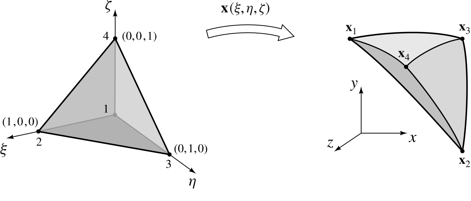
Fig. 3.13 The master tetrahedron element is mapped to its image in physical coordinates  .
.
The Gauss quadrature rule for the 3D Tetrahedron given in Table 3.1 is used to integrate this element. The shape functions are
(3.180)
3.9.2.5. 3D Triangular Face Element
The tetrahedral element presented in 3D Tetrahedron Element has three-node, triangular faces, which are topologically equivalent to the two-dimensional triangular element that was presented in 2D Triangular Element. Accordingly, the shape functions are identical (3.177). The Gauss quadrature rule for the 2D Triangle that is given in Table 3.1 is used to integrate this element.
Since the physical coordinates are three-dimensional, but there are only two parameters on the surface, , the transformation from computational coordinates to physical coordinates requires a little elaboration. Vector calculus provides a formula for the integral of a scalar function over a parameterized surface [28]. We are interested in the surface integral
(3.181)
where  is the three dimensional surface of our face element, and is given by the isoparametric mapping
(3.182)
It can be shown that (3.181) may be computed as
(3.183)
where  is the master element,
  , and the determinant of the Jacobian matrix may be written as
(3.184)
Equation (3.184) involves the calculation of the determinants of three sub-matrices. For example,

3.9.2.6. 3D Hexahedron Element
Fig. 3.14 shows the topology of the eight-node, linear hexahedral master element.
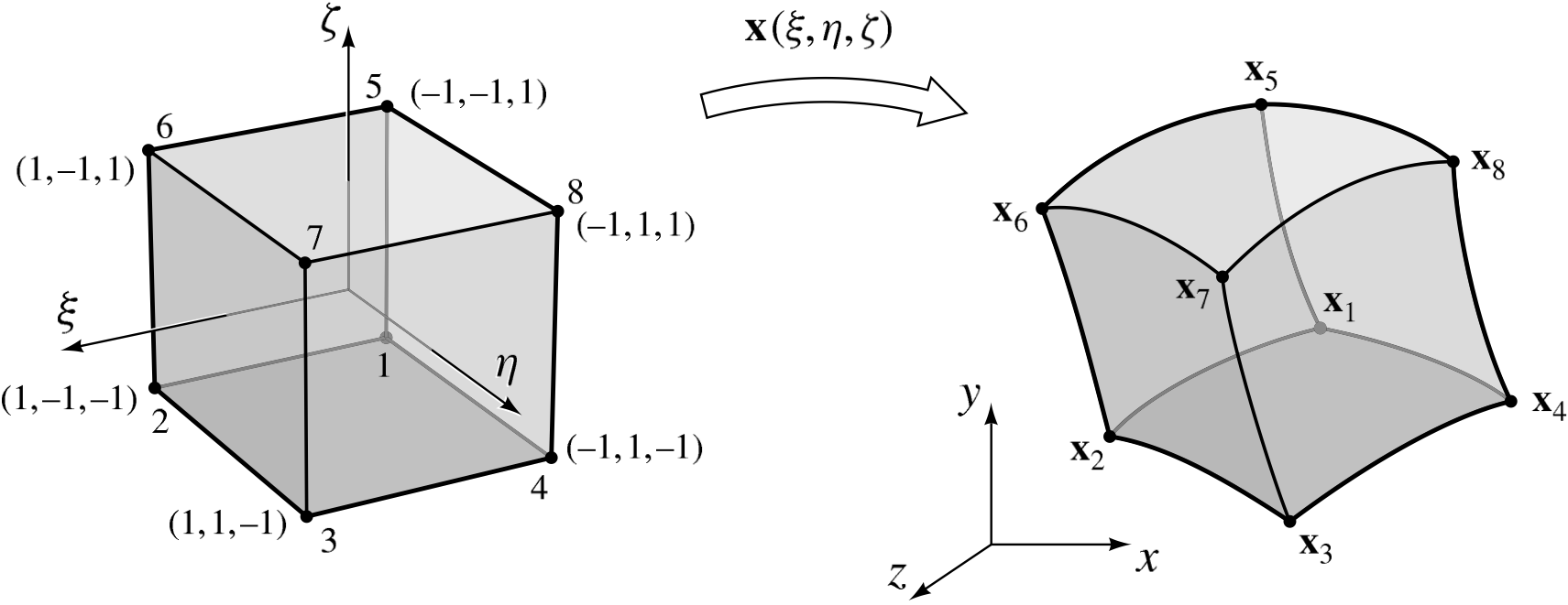
Fig. 3.14 The master hexahedron element in  on the region
 ![[-1,1]\times[-1,1]\times[-1,1]](data:image/svg+xml;base64,PD94bWwgdmVyc2lvbj0nMS4wJyBlbmNvZGluZz0nVVRGLTgnPz4KPCEtLSBUaGlzIGZpbGUgd2FzIGdlbmVyYXRlZCBieSBkdmlzdmdtIDMuMC4zIC0tPgo8c3ZnIHZlcnNpb249JzEuMScgeG1sbnM9J2h0dHA6Ly93d3cudzMub3JnLzIwMDAvc3ZnJyB4bWxuczp4bGluaz0naHR0cDovL3d3dy53My5vcmcvMTk5OS94bGluaycgd2lkdGg9JzE0OC43MjYyMzlwdCcgaGVpZ2h0PScxMy45NDc2OTZwdCcgdmlld0JveD0nMCAtMTAuNDYwNzcyIDE0OC43MjYyMzkgMTMuOTQ3Njk2Jz4KPGRlZnM+CjxwYXRoIGlkPSdnMS01OScgZD0nTTIuNzE5ODAxIC4wNTU3OTFDMi43MTk4MDEtLjc1MzE3NiAyLjQ1NDc5NS0xLjM1MjkyNyAxLjg4MjkzOS0xLjM1MjkyN0MxLjQzNjYxMy0xLjM1MjkyNyAxLjIxMzQ1LS45OTAyODYgMS4yMTM0NS0uNjgzNDM3UzEuNDIyNjY1IDAgMS44OTY4ODcgMEMyLjA3ODIwNyAwIDIuMjMxNjMxLS4wNTU3OTEgMi4zNTcxNjEtLjE4MTMyQzIuMzg1MDU2LS4yMDkyMTUgMi4zOTkwMDQtLjIwOTIxNSAyLjQxMjk1MS0uMjA5MjE1QzIuNDQwODQ3LS4yMDkyMTUgMi40NDA4NDctLjAxMzk0OCAyLjQ0MDg0NyAuMDU1NzkxQzIuNDQwODQ3IC41MTYwNjUgMi4zNTcxNjEgMS40MjI2NjUgMS41NDgxOTQgMi4zMjkyNjVDMS4zOTQ3NyAyLjQ5NjYzOCAxLjM5NDc3IDIuNTI0NTMzIDEuMzk0NzcgMi41NTI0MjhDMS4zOTQ3NyAyLjYyMjE2NyAxLjQ2NDUwOCAyLjY5MTkwNSAxLjUzNDI0NyAyLjY5MTkwNUMxLjY0NTgyOCAyLjY5MTkwNSAyLjcxOTgwMSAxLjY1OTc3NiAyLjcxOTgwMSAuMDU1NzkxWicvPgo8cGF0aCBpZD0nZzItNDknIGQ9J000LjAxNjkzNi04Ljk0MDQ3M0M0LjAxNjkzNi05LjI2MTI3IDQuMDE2OTM2LTkuMjc1MjE4IDMuNzM3OTgzLTkuMjc1MjE4QzMuNDAzMjM4LTguODk4NjMgMi43MDU4NTMtOC4zODI1NjUgMS4yNjkyNC04LjM4MjU2NVYtNy45NzgwODJDMS41OTAwMzctNy45NzgwODIgMi4yODc0MjItNy45NzgwODIgMy4wNTQ1NDUtOC4zNDA3MjJWLTEuMDczOTczQzMuMDU0NTQ1LS41NzE4NTYgMy4wMTI3MDItLjQwNDQ4MyAxLjc4NTMwNS0uNDA0NDgzSDEuMzUyOTI3VjBDMS43Mjk1MTQtLjAyNzg5NSAzLjA4MjQ0MS0uMDI3ODk1IDMuNTQyNzE1LS4wMjc4OTVTNS4zNDE5NjgtLjAyNzg5NSA1LjcxODU1NSAwVi0uNDA0NDgzSDUuMjg2MTc3QzQuMDU4NzgtLjQwNDQ4MyA0LjAxNjkzNi0uNTcxODU2IDQuMDE2OTM2LTEuMDczOTczVi04Ljk0MDQ3M1onLz4KPHBhdGggaWQ9J2cyLTkxJyBkPSdNMy40ODY5MjQgMy40ODY5MjRWMi45NzA4NTlIMi4xMzM5OThWLTkuOTQ0NzA3SDMuNDg2OTI0Vi0xMC40NjA3NzJIMS42MTc5MzNWMy40ODY5MjRIMy40ODY5MjRaJy8+CjxwYXRoIGlkPSdnMi05MycgZD0nTTIuMTYxODkzLTEwLjQ2MDc3MkguMjkyOTAyVi05Ljk0NDcwN0gxLjY0NTgyOFYyLjk3MDg1OUguMjkyOTAyVjMuNDg2OTI0SDIuMTYxODkzVi0xMC40NjA3NzJaJy8+CjxwYXRoIGlkPSdnMC0wJyBkPSdNOS4xOTE1MzItMy4yMDc5N0M5LjQyODY0My0zLjIwNzk3IDkuNjc5NzAxLTMuMjA3OTcgOS42Nzk3MDEtMy40ODY5MjRTOS40Mjg2NDMtMy43NjU4NzggOS4xOTE1MzItMy43NjU4NzhIMS42NDU4MjhDMS40MDg3MTctMy43NjU4NzggMS4xNTc2NTktMy43NjU4NzggMS4xNTc2NTktMy40ODY5MjRTMS40MDg3MTctMy4yMDc5NyAxLjY0NTgyOC0zLjIwNzk3SDkuMTkxNTMyWicvPgo8cGF0aCBpZD0nZzAtMicgZD0nTTUuNDI1NjU0LTMuODc3NDZMMi42MzYxMTUtNi42NTMwNTFDMi40Njg3NDItNi44MjA0MjMgMi40NDA4NDctNi44NDgzMTkgMi4zMjkyNjUtNi44NDgzMTlDMi4xODk3ODgtNi44NDgzMTkgMi4wNTAzMTEtNi43MjI3OSAyLjA1MDMxMS02LjU2OTM2NUMyLjA1MDMxMS02LjQ3MTczMSAyLjA3ODIwNy02LjQ0MzgzNiAyLjIzMTYzMS02LjI5MDQxMUw1LjAyMTE3MS0zLjQ4NjkyNEwyLjIzMTYzMS0uNjgzNDM3QzIuMDc4MjA3LS41MzAwMTIgMi4wNTAzMTEtLjUwMjExNyAyLjA1MDMxMS0uNDA0NDgzQzIuMDUwMzExLS4yNTEwNTkgMi4xODk3ODgtLjEyNTUyOSAyLjMyOTI2NS0uMTI1NTI5QzIuNDQwODQ3LS4xMjU1MjkgMi40Njg3NDItLjE1MzQyNSAyLjYzNjExNS0uMzIwNzk3TDUuNDExNzA2LTMuMDk2Mzg5TDguMjk4ODc5LS4yMDkyMTVDOC4zMjY3NzUtLjE5NTI2OCA4LjQyNDQwOC0uMTI1NTI5IDguNTA4MDk1LS4xMjU1MjlDOC42NzU0NjctLjEyNTUyOSA4Ljc4NzA0OS0uMjUxMDU5IDguNzg3MDQ5LS40MDQ0ODNDOC43ODcwNDktLjQzMjM3OSA4Ljc4NzA0OS0uNDg4MTY5IDguNzQ1MjA1LS41NTc5MDhDOC43MzEyNTgtLjU4NTgwMyA2LjUxMzU3NC0yLjc3NTU5MiA1LjgxNjE4OS0zLjQ4NjkyNEw4LjM2ODYxOC02LjAzOTM1MkM4LjQzODM1Ni02LjEyMzAzOSA4LjY0NzU3Mi02LjMwNDM1OSA4LjcxNzMxLTYuMzg4MDQ1QzguNzMxMjU4LTYuNDE1OTQgOC43ODcwNDktNi40NzE3MzEgOC43ODcwNDktNi41NjkzNjVDOC43ODcwNDktNi43MjI3OSA4LjY3NTQ2Ny02Ljg0ODMxOSA4LjUwODA5NS02Ljg0ODMxOUM4LjM5NjUxMy02Ljg0ODMxOSA4LjM0MDcyMi02Ljc5MjUyOCA4LjE4NzI5OC02LjYzOTEwM0w1LjQyNTY1NC0zLjg3NzQ2WicvPgo8L2RlZnM+CjxnIGlkPSdwYWdlMSc+Cjx1c2UgeD0nMCcgeT0nMCcgeGxpbms6aHJlZj0nI2cyLTkxJy8+Cjx1c2UgeD0nMy43OTM2MDUnIHk9JzAnIHhsaW5rOmhyZWY9JyNnMC0wJy8+Cjx1c2UgeD0nMTQuNjQxODUxJyB5PScwJyB4bGluazpocmVmPScjZzItNDknLz4KPHVzZSB4PScyMS40NzAzNCcgeT0nMCcgeGxpbms6aHJlZj0nI2cxLTU5Jy8+Cjx1c2UgeD0nMjcuNTg4NTQxJyB5PScwJyB4bGluazpocmVmPScjZzItNDknLz4KPHVzZSB4PSczNC40MTcwMjknIHk9JzAnIHhsaW5rOmhyZWY9JyNnMi05MycvPgo8dXNlIHg9JzQxLjMxMDA5NScgeT0nMCcgeGxpbms6aHJlZj0nI2cwLTInLz4KPHVzZSB4PSc1NS4yNTc4MDInIHk9JzAnIHhsaW5rOmhyZWY9JyNnMi05MScvPgo8dXNlIHg9JzU5LjA1MTQwNycgeT0nMCcgeGxpbms6aHJlZj0nI2cwLTAnLz4KPHVzZSB4PSc2OS44OTk2NTQnIHk9JzAnIHhsaW5rOmhyZWY9JyNnMi00OScvPgo8dXNlIHg9Jzc2LjcyODE0MicgeT0nMCcgeGxpbms6aHJlZj0nI2cxLTU5Jy8+Cjx1c2UgeD0nODIuODQ2MzQzJyB5PScwJyB4bGluazpocmVmPScjZzItNDknLz4KPHVzZSB4PSc4OS42NzQ4MzInIHk9JzAnIHhsaW5rOmhyZWY9JyNnMi05MycvPgo8dXNlIHg9Jzk2LjU2Nzg5NycgeT0nMCcgeGxpbms6aHJlZj0nI2cwLTInLz4KPHVzZSB4PScxMTAuNTE1NjA1JyB5PScwJyB4bGluazpocmVmPScjZzItOTEnLz4KPHVzZSB4PScxMTQuMzA5MjEnIHk9JzAnIHhsaW5rOmhyZWY9JyNnMC0wJy8+Cjx1c2UgeD0nMTI1LjE1NzQ1NicgeT0nMCcgeGxpbms6aHJlZj0nI2cyLTQ5Jy8+Cjx1c2UgeD0nMTMxLjk4NTk0NScgeT0nMCcgeGxpbms6aHJlZj0nI2cxLTU5Jy8+Cjx1c2UgeD0nMTM4LjEwNDE0NScgeT0nMCcgeGxpbms6aHJlZj0nI2cyLTQ5Jy8+Cjx1c2UgeD0nMTQ0LjkzMjYzNCcgeT0nMCcgeGxpbms6aHJlZj0nI2cyLTkzJy8+CjwvZz4KPC9zdmc+CjwhLS0gREVQVEg9NSAtLT4=) is mapped to its image in physical coordinates .
is mapped to its image in physical coordinates .
The Gauss quadrature rule for the 3D Hexahedron that is given in Table 3.1 is used to integrate this element. The shape functions are

3.9.2.7. 3D Quadrilateral Face Element
The hexahedron element described in 3D Hexahedron Element has quadrilateral faces. The shape functions that are used for interpolating on one of these faces are identical to the shape functions used for the 2D Quadrilateral Element in (3.178). As discussed in 3D Triangular Face Element, integrals on this surface master element may be computed according to (3.183), with the determinant given by (3.184). The Gauss quadrature rule for the 2D Quadrilateral that is given in Table 3.1 is used to integrate this element.
3.9.2.8. 3D Triangular Shell Element
Beta Capability
Shell support in Aria is currently a beta feature. This capability is a work-in-progress and is not thoroughly tested and should be used with caution.
Sometimes, a subdomain  may be very thin, and may also possibly consist of a highly conductive material like aluminum. In this case, it is reasonable to neglect the thermal gradient through the thickness of
  . Shell elements are specialized volume elements that are often used to model this situation. The topology of the linear triangular shell is illustrated in Fig. 3.15, which has three nodes, and two faces. Topologically, the shell has no thickness that can be derived solely from its node coordinates; instead, the thickness is an attribute specified as input data. The shape functions are identical to (3.177) in 2D Triangular Element.
The transformation from computational coordinates to physical coordinates for the three-dimensional shell element depends on the thickness attribute. In this case, we wish to calculate the volume integral
(3.185)
The parametric mapping from computational coordinates to physical coordinates may be regarded as the surface mapping, plus a component that comes up out of the shell mid-plane. With reference to Fig. 3.15, we may write this mapping as
(3.186)
where the shape functions are given by (3.177),  ,
,  denotes the thickness of the shell at node ,
 ![\zeta \in [-1,1]](data:image/svg+xml;base64,PD94bWwgdmVyc2lvbj0nMS4wJyBlbmNvZGluZz0nVVRGLTgnPz4KPCEtLSBUaGlzIGZpbGUgd2FzIGdlbmVyYXRlZCBieSBkdmlzdmdtIDMuMC4zIC0tPgo8c3ZnIHZlcnNpb249JzEuMScgeG1sbnM9J2h0dHA6Ly93d3cudzMub3JnLzIwMDAvc3ZnJyB4bWxuczp4bGluaz0naHR0cDovL3d3dy53My5vcmcvMTk5OS94bGluaycgd2lkdGg9JzYyLjI3NTk4OHB0JyBoZWlnaHQ9JzEzLjk0NzY5NnB0JyB2aWV3Qm94PScwIC0xMC40NjA3NzIgNjIuMjc1OTg4IDEzLjk0NzY5Nic+CjxkZWZzPgo8cGF0aCBpZD0nZzItNDknIGQ9J000LjAxNjkzNi04Ljk0MDQ3M0M0LjAxNjkzNi05LjI2MTI3IDQuMDE2OTM2LTkuMjc1MjE4IDMuNzM3OTgzLTkuMjc1MjE4QzMuNDAzMjM4LTguODk4NjMgMi43MDU4NTMtOC4zODI1NjUgMS4yNjkyNC04LjM4MjU2NVYtNy45NzgwODJDMS41OTAwMzctNy45NzgwODIgMi4yODc0MjItNy45NzgwODIgMy4wNTQ1NDUtOC4zNDA3MjJWLTEuMDczOTczQzMuMDU0NTQ1LS41NzE4NTYgMy4wMTI3MDItLjQwNDQ4MyAxLjc4NTMwNS0uNDA0NDgzSDEuMzUyOTI3VjBDMS43Mjk1MTQtLjAyNzg5NSAzLjA4MjQ0MS0uMDI3ODk1IDMuNTQyNzE1LS4wMjc4OTVTNS4zNDE5NjgtLjAyNzg5NSA1LjcxODU1NSAwVi0uNDA0NDgzSDUuMjg2MTc3QzQuMDU4NzgtLjQwNDQ4MyA0LjAxNjkzNi0uNTcxODU2IDQuMDE2OTM2LTEuMDczOTczVi04Ljk0MDQ3M1onLz4KPHBhdGggaWQ9J2cyLTkxJyBkPSdNMy40ODY5MjQgMy40ODY5MjRWMi45NzA4NTlIMi4xMzM5OThWLTkuOTQ0NzA3SDMuNDg2OTI0Vi0xMC40NjA3NzJIMS42MTc5MzNWMy40ODY5MjRIMy40ODY5MjRaJy8+CjxwYXRoIGlkPSdnMi05MycgZD0nTTIuMTYxODkzLTEwLjQ2MDc3MkguMjkyOTAyVi05Ljk0NDcwN0gxLjY0NTgyOFYyLjk3MDg1OUguMjkyOTAyVjMuNDg2OTI0SDIuMTYxODkzVi0xMC40NjA3NzJaJy8+CjxwYXRoIGlkPSdnMS0xNicgZD0nTTIuNjM2MTE1LS42ODM0MzdDMS44MTMyLTEuMDA0MjM0IDEuMzM4OTc5LTEuNjMxODggMS4zMzg5NzktMi42Nzc5NThDMS4zMzg5NzktNC41ODg3OTIgMi43NDc2OTYtNy4xNDEyMiA0LjQ2MzI2My04LjEzMTUwN0M0LjcxNDMyMS03Ljg5NDM5NiA1LjAzNTExOC03Ljg5NDM5NiA1LjMwMDEyNS03Ljg5NDM5NkM1LjY0ODgxNy03Ljg5NDM5NiA2LjQ5OTYyNi03Ljg5NDM5NiA2LjQ5OTYyNi04LjI5ODg3OUM2LjQ5OTYyNi04LjYzMzYyNCA1Ljg3MTk4LTguNjQ3NTcyIDUuNDI1NjU0LTguNjQ3NTcyQzUuMTQ2Ny04LjY0NzU3MiA0LjkwOTU4OS04LjY0NzU3MiA0LjU0Njk0OS04LjQ5NDE0N0M0LjQ2MzI2My04LjY3NTQ2NyA0LjQyMTQyLTguODcwNzM1IDQuNDIxNDItOS4wNzk5NUM0LjQyMTQyLTkuMzMxMDA5IDQuNDc3MjEtOS41MjYyNzYgNC40NzcyMS05LjU2ODEyQzQuNDc3MjEtOS42NTE4MDYgNC40MDc0NzItOS43MDc1OTcgNC4zMzc3MzMtOS43MDc1OTdDNC4xMTQ1Ny05LjcwNzU5NyA0LjExNDU3LTkuMTkxNTMyIDQuMTE0NTctOS4wNzk5NUM0LjExNDU3LTguOTU0NDIxIDQuMTE0NTctOC42NjE1MTkgNC4yODE5NDMtOC4zNjg2MThDMi42NjQwMS03LjUzMTc1NiAuNjI3NjQ2LTQuOTIzNTM3IC42Mjc2NDYtMi4zMTUzMThDLjYyNzY0Ni0uNDA0NDgzIDEuODk2ODg3IC4wNDE4NDMgMi42MjIxNjcgLjI5MjkwMkMyLjgwMzQ4NyAuMzQ4NjkyIDMuMjQ5ODEzIC41MDIxMTcgMy40MzExMzMgLjU3MTg1NkM0LjAwMjk4OSAuNzY3MTIzIDQuNTQ2OTQ5IC45NDg0NDMgNC41NDY5NDkgMS42MTc5MzNDNC41NDY5NDkgMi4wMjI0MTYgNC4yNTQwNDcgMi41NjYzNzYgMy43Mzc5ODMgMi41NjYzNzZDMy40NTkwMjkgMi41NjYzNzYgMy4wODI0NDEgMi40Njg3NDIgMi43MzM3NDggMi4xMjAwNUMyLjY3Nzk1OCAyLjA2NDI1OSAyLjY1MDA2MiAyLjAzNjM2NCAyLjU4MDMyNCAyLjAzNjM2NEMyLjQ2ODc0MiAyLjAzNjM2NCAyLjQ0MDg0NyAyLjE0Nzk0NSAyLjQ0MDg0NyAyLjE3NTg0MUMyLjQ0MDg0NyAyLjMxNTMxOCAzLjA0MDU5OCAyLjg0NTMzIDMuNzM3OTgzIDIuODQ1MzNDNC42MzA2MzUgMi44NDUzMyA1LjI0NDMzNCAxLjkxMDgzNCA1LjI0NDMzNCAxLjE4NTU1NEM1LjI0NDMzNCAuMjA5MjE1IDQuNDM1MzY3LS4wNjk3MzggMy45MTkzMDMtLjIzNzExMUwyLjYzNjExNS0uNjgzNDM3Wk00Ljc3MDExMi04LjI3MDk4NEM0Ljk3OTMyOC04LjM2ODYxOCA1LjE3NDU5NS04LjM2ODYxOCA1LjQxMTcwNi04LjM2ODYxOEM1Ljg1ODAzMi04LjM2ODYxOCA1Ljg5OTg3NS04LjM1NDY3IDYuMTc4ODI5LTguMjg0OTMyQzYuMDExNDU3LTguMjE1MTkzIDUuODk5ODc1LTguMTczMzUgNS4zMTQwNzItOC4xNzMzNUM1LjAyMTE3MS04LjE3MzM1IDQuOTIzNTM3LTguMTczMzUgNC43NzAxMTItOC4yNzA5ODRaJy8+CjxwYXRoIGlkPSdnMS01OScgZD0nTTIuNzE5ODAxIC4wNTU3OTFDMi43MTk4MDEtLjc1MzE3NiAyLjQ1NDc5NS0xLjM1MjkyNyAxLjg4MjkzOS0xLjM1MjkyN0MxLjQzNjYxMy0xLjM1MjkyNyAxLjIxMzQ1LS45OTAyODYgMS4yMTM0NS0uNjgzNDM3UzEuNDIyNjY1IDAgMS44OTY4ODcgMEMyLjA3ODIwNyAwIDIuMjMxNjMxLS4wNTU3OTEgMi4zNTcxNjEtLjE4MTMyQzIuMzg1MDU2LS4yMDkyMTUgMi4zOTkwMDQtLjIwOTIxNSAyLjQxMjk1MS0uMjA5MjE1QzIuNDQwODQ3LS4yMDkyMTUgMi40NDA4NDctLjAxMzk0OCAyLjQ0MDg0NyAuMDU1NzkxQzIuNDQwODQ3IC41MTYwNjUgMi4zNTcxNjEgMS40MjI2NjUgMS41NDgxOTQgMi4zMjkyNjVDMS4zOTQ3NyAyLjQ5NjYzOCAxLjM5NDc3IDIuNTI0NTMzIDEuMzk0NzcgMi41NTI0MjhDMS4zOTQ3NyAyLjYyMjE2NyAxLjQ2NDUwOCAyLjY5MTkwNSAxLjUzNDI0NyAyLjY5MTkwNUMxLjY0NTgyOCAyLjY5MTkwNSAyLjcxOTgwMSAxLjY1OTc3NiAyLjcxOTgwMSAuMDU1NzkxWicvPgo8cGF0aCBpZD0nZzAtMCcgZD0nTTkuMTkxNTMyLTMuMjA3OTdDOS40Mjg2NDMtMy4yMDc5NyA5LjY3OTcwMS0zLjIwNzk3IDkuNjc5NzAxLTMuNDg2OTI0UzkuNDI4NjQzLTMuNzY1ODc4IDkuMTkxNTMyLTMuNzY1ODc4SDEuNjQ1ODI4QzEuNDA4NzE3LTMuNzY1ODc4IDEuMTU3NjU5LTMuNzY1ODc4IDEuMTU3NjU5LTMuNDg2OTI0UzEuNDA4NzE3LTMuMjA3OTcgMS42NDU4MjgtMy4yMDc5N0g5LjE5MTUzMlonLz4KPHBhdGggaWQ9J2cwLTUwJyBkPSdNNy42NDMzMzctMy4yMDc5N0M3Ljg4MDQ0OC0zLjIwNzk3IDguMTMxNTA3LTMuMjA3OTcgOC4xMzE1MDctMy40ODY5MjRTNy44ODA0NDgtMy43NjU4NzggNy42NDMzMzctMy43NjU4NzhIMS43Mjk1MTRDMS44OTY4ODctNS42MzQ4NjkgMy41MDA4NzItNi45NzM4NDggNS40Njc0OTctNi45NzM4NDhINy42NDMzMzdDNy44ODA0NDgtNi45NzM4NDggOC4xMzE1MDctNi45NzM4NDggOC4xMzE1MDctNy4yNTI4MDJTNy44ODA0NDgtNy41MzE3NTYgNy42NDMzMzctNy41MzE3NTZINS40Mzk2MDFDMy4wNTQ1NDUtNy41MzE3NTYgMS4xNTc2NTktNS43MTg1NTUgMS4xNTc2NTktMy40ODY5MjRTMy4wNTQ1NDUgLjU1NzkwOCA1LjQzOTYwMSAuNTU3OTA4SDcuNjQzMzM3QzcuODgwNDQ4IC41NTc5MDggOC4xMzE1MDcgLjU1NzkwOCA4LjEzMTUwNyAuMjc4OTU0UzcuODgwNDQ4IDAgNy42NDMzMzcgMEg1LjQ2NzQ5N0MzLjUwMDg3MiAwIDEuODk2ODg3LTEuMzM4OTc5IDEuNzI5NTE0LTMuMjA3OTdINy42NDMzMzdaJy8+CjwvZGVmcz4KPGcgaWQ9J3BhZ2UxJz4KPHVzZSB4PScwJyB5PScwJyB4bGluazpocmVmPScjZzEtMTYnLz4KPHVzZSB4PScxMC44OTI1MzMnIHk9JzAnIHhsaW5rOmhyZWY9JyNnMC01MCcvPgo8dXNlIHg9JzI0LjA2NTM1NScgeT0nMCcgeGxpbms6aHJlZj0nI2cyLTkxJy8+Cjx1c2UgeD0nMjcuODU4OTU5JyB5PScwJyB4bGluazpocmVmPScjZzAtMCcvPgo8dXNlIHg9JzM4LjcwNzIwNicgeT0nMCcgeGxpbms6aHJlZj0nI2cyLTQ5Jy8+Cjx1c2UgeD0nNDUuNTM1Njk0JyB5PScwJyB4bGluazpocmVmPScjZzEtNTknLz4KPHVzZSB4PSc1MS42NTM4OTUnIHk9JzAnIHhsaW5rOmhyZWY9JyNnMi00OScvPgo8dXNlIHg9JzU4LjQ4MjM4NCcgeT0nMCcgeGxpbms6aHJlZj0nI2cyLTkzJy8+CjwvZz4KPC9zdmc+CjwhLS0gREVQVEg9NSAtLT4=) is the parametric coordinate in the direction locally orthogonal to the shell mid-plane, and we have defined the inner products
is the parametric coordinate in the direction locally orthogonal to the shell mid-plane, and we have defined the inner products
(3.187)
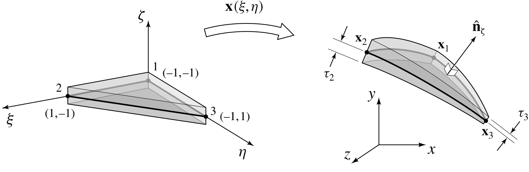
Fig. 3.15 The midplane of the master triangular shell element is mapped to its image in physical coordinates , and the variation in the shell thickness is represented with the element shape functions.
In (3.187),  is the unit vector in the direction locally orthogonal to the element mid-plane, and
  and
and  are the unit vectors in the
  and
and  coordinate directions, respectively. The volume integral in (3.185) on the master element is
(3.188)
where is the determinant of the Jacobian matrix obtained from the transformation given by (3.186).
Aria currently only supports constant thickness shells. In this case,  reduces to
(3.189)
where  is the constant shell thickness, denotes the triangular surface of the shell mid-plane, is the determinant of the transformation given by (3.182), and the Gauss quadrature rule for the 2D Triangle that is given in Table 3.1 is used to perform the numerical integration.
3.9.2.9. 3D Quadrilateral Shell Element
Beta Capability
Shell support in Aria is currently a beta feature. This capability is a work-in-progress and is not thoroughly tested and should be used with caution.
The three-dimensional, linear, quadrilateral shell element is, in principle, no different from the triangular shell element which we discussed in 3D Triangular Shell Element. As illustrated in Fig. 3.16, the quadrilateral shell has four nodes, instead of three, with the basis functions given in (3.178). The transformation from computational coordinates to physical coordinates is again given by (3.186), but with  , and the are defined by (3.178).
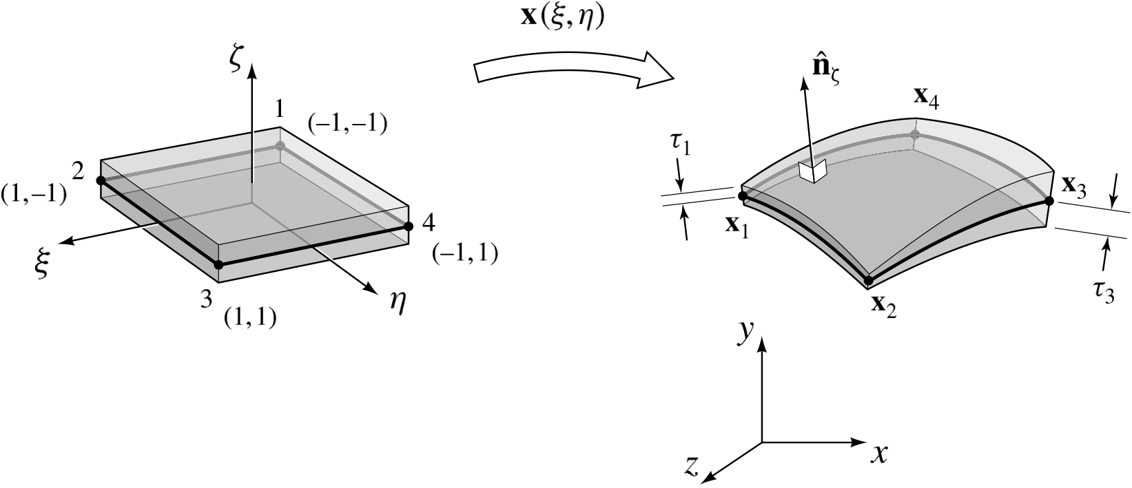
Fig. 3.16 The midplane of the master quadrilateral shell element is mapped to its image in physical coordinates , and the variation in the shell thickness is represented with the element shape functions.
Currently, Aria only supports constant thickness shells, and the simplifications discussed in 3D Triangular Shell Element also apply in this case. The volume integral therefore reduces to the product of the shell thickness and the integral over the mid-plane surface, with the transformation from computational to physical coordinates identical to that which is described in 2D Quadrilateral Element.