2.1. SIERRA Scope

These commands are used to set up some of the fundamentals of the Sierra/SM input. The commands are physics independent, or at least can be shared between physics. The commands lie in the SIERRA scope, not in the procedure or region scope.

2.1.1. SIERRA Command Block

BEGIN SIERRA <string>name
  #
  # All other command blocks and command lines
  # appear within the SIERRA scope defined by
  # begin/end sierra.
  #
END [SIERRA <string>name]

All input commands must occur within a SIERRA command block. The syntax for beginning the command block is:

BEGIN SIERRA <string>name

and for terminating the command block is as follows:

END [SIERRA <string>name]

In these input lines, name is a name for the SIERRA command block. All other commands for the analysis must be within this command block structure. The name for the SIERRA command block is often a descriptive name that identifies the analysis. The name is not currently used anywhere else in the file and is completely arbitrary.

2.1.2. Title

TITLE <string list>title

To permit a fuller description of the analysis, the input has a TITLE command line for the analysis, where title is a text description of the analysis. The title is transferred to the results file.

2.1.3. Restart Control

Restart allows a user to resume an analysis by initializing all of its fields from a specific time of a previous simulation. For more background information on restart, see Section 9.9.

The time at which to restart an analysis can be specified in either the Sierra scope or the RESTART DATA command block in the region scope. If the restart time is specified in the Sierra scope, a RESTART DATA command block is still required to specify input and output restart data filenames. When performing a multi-physics simulation involving coupling Sierra/SM to another Sierra code, it is beneficial to specify the restart time in the Sierra scope. However, if the analysis involves only Sierra/SM, it is sufficient to specify a restart time only in the RESTART DATA command block.

If using restart commands in the Sierra scope, one of two restart command lines (RESTART or RESTART TIME) are used. The details of these two commands are described below:

2.1.3.1. Restart Time

RESTART TIME = <real>restart_time

The RESTART TIME command line specifies a time from which to restart the simulation. This restart option will pick the restart time on the restart file that is closest to the user-specified time in the RESTART TIME command line. If the user specifies a restart time greater than the last time written to a restart file, the last time written to the restart file is picked as the restart time. If this command is specified, a restart file must exist. If the input restart database does not exist, the code will exit with an error. For details of this feature and a use case example, see Section 9.9.1.3.

Using the RESTART TIME command requires the user to be more active in the management of the file names to prevent the overwriting of restart, results, and history files. To prevent the overwriting of existing restart files, an input restart file and an output restart file can be specified in the RESTART DATA command block. To prevent the overwriting of results and history files, the filenames must be changed in the respective output blocks. It is best to break the analysis into a sequence of “restart runs” where each ‘restart run’ will consist of its own restart, results, and history files. For more information on overwriting of output files, see Section 9. If the user would prefer not to manage the overwriting of files, the automatic restart feature should be used. This feature is outlined below in Section 2.1.3.2.

2.1.3.2. Automatic Restart

RESTART = AUTOMATIC|AUTO

The AUTOMATIC or AUTO restart option automatically selects the last time written to the last restart file as the restart time. The automatic restart feature allows the user to restart runs with minimal changes to the input file. The only quantity that must be changed to move from one restart to another is the termination time. The RESTART command line manages the restart files to ensure any previous restart files are not overwritten. It also manages the results and history files to ensure any previous results or history files are not overwritten as well. For details of this feature and a use case example, see Section 9.9.1.2.

If the AUTOMATIC option is used and the restart database does not exist, the analysis will start from the initial time and not read any restart data. Note, the path to the restart file must be carefully defined when using the AUTOMATIC option. If there is a typo in the path or file name that prevents the correct restart database from being found, the analysis will start from the beginning of the first time period without error.

See Section 9.9 for a full discussion of implementing the restart capability.

2.1.4. User Subroutine Identification

USER SUBROUTINE FILE = <string>file_name

This command line is a part of a set of commands that are used to implement the user subroutine functionality. The string file_name identifies the name of the file that contains the FORTRAN code of one or more user subroutines.

To understand how this command line is used, see Section 10.2.

2.1.5. XY Functions

BEGIN FUNCTION <string>function_name
  TYPE = <string>CONSTANT|PIECEWISE LINEAR|PIECEWISE CONSTANT|
    ANALYTIC|PIECEWISE ANALYTIC|MULTICOLUMN PIECEWISE LINEAR|
    PIECEWISE MULTIVARIATE
  EXPRESSION VARIABLE: <var_name> = NODAL|NODAL_VECTOR|
    NODAL_TENSOR|NODAL_SYM_TENSOR|ELEMENT|ELEMENT_VECTOR|
    ELEMENT_TENSOR|ELEMENT_SYM_TENSOR|FACE|
    GLOBAL <var_source>
  ABSCISSA = <string>abscissa_label
  ORDINATE = <string>ordinate_label
  X SCALE = <real>x_scale(1.0)
  X OFFSET = <real>x_offset(0.0)
  Y SCALE = <real>y_scale(1.0)
  Y OFFSET = <real>y_offset(0.0)
  ABSCISSA SCALE = <real>x_scale(1.0)
  ABSCISSA OFFSET = <real>x_offset(0.0)
  ORDINATE SCALE = <real>y_scale(1.0)
  ORDINATE OFFSET = <real>y_offset(0.0)
  COLUMN TITLES = <string> <string> ...
  FIELD TYPES = GLOBAL|NODAL|ELEMENT GLOBAL|NODAL|ELEMENT ...
  BEGIN VALUES
    <real>x_1   <real>y_1
    <real>x_2   <real>y_2
    ...
    <real>x_n   <real>y_n
  END [VALUES]
  BEGIN EXPRESSIONS
    <real>x_1   <string>analytic_expression_1
    <real>x_2   <string>analytic_expression_2
    ...
    <real>x_n   <string>analytic_expression_n
  END
  DATA FILE = <string>fileName
    [X FROM COLUMN <int>xCol Y FROM COLUMN <int>yCol]
  AT DISCONTINUITY EVALUATE TO <string>LEFT|RIGHT(LEFT)
  EVALUATE EXPRESSION = <string>analytic_expression1;
    analytic_expression2; ...
  DIFFERENTIATE EXPRESSION = <string>analytic_expression1;
    analytic_expression2; ...
  EVALUATE FROM <real> TO <real> BY <real>
  DEBUG = ON|OFF(OFF)
END [FUNCTION <string>function_name]

Many Sierra/SM features are driven by a user-defined description of the dependence of one variable on another. For instance, the prescribed displacement boundary condition requires the definition of a time-versus-displacement relation, and the thermal strain computations require the definition of a thermal-strain-versus-temperature relation. SIERRA provides a general method of defining these relations as functions using the FUNCTION command block, as shown above.

Many options exist for defining a general X versus Y function. More limited options exist for defining more complex functions of multiple variables. The more complex functions are described in Section 2.1.6.

There is no limit to the number of functions that can be defined. All function definitions must appear within the SIERRA scope.

A description of the various parts of the FUNCTION command block follows:

• The string function_name is a user-selected name for the function that is unique to the function definitions within the input file. This name is used to refer to this function in other locations in the input file.

• The TYPE command line has seven options to define the type of function. The value of this string can be CONSTANT, PIECEWISE LINEAR, PIECEWISE CONSTANT, ANALYTIC, PIECEWISE ANALYTIC, MULTICOLUMN PIECEWISE LINEAR, or PIECEWISE MULTIVARIATE.

• The ABSCISSA command line provides a descriptive label for the independent variable (\(x\)-axis) with the string abscissa_label. This command line is optional. (Note: Previous versions of SIERRA allowed the user to optionally add a scale factor and/or an offset via the SCALE and OFFSET keywords. These keywords are deprecated and their use will generate a parse error. Any desired scale factors and offsets need to be specified via the X SCALE and/or X OFFSET command lines, respectively.)

• The ORDINATE command line provides a descriptive label for the dependent variable (\(y\)-axis) with the string ordinate_label. This command line is optional. (Note: Previous versions of SIERRA allowed the user to optionally add a scale factor and/or an offset via the SCALE and OFFSET keywords. These keywords are deprecated and their use will generate a parse error. Any desired scale factors and offsets need to be specified via the Y SCALE and/or Y OFFSET command lines, respectively.)

• The X SCALE command line sets the scale factor value for the abscissa, which has the following effect: \(\textit{abscissa}_{\textit{scaled,offset}} = \textit{scale} * (\textit{abscissa} + \textit{offset})\). (Note: If no offset is specified via X OFFSET, \(\textit{offset} = 0.0\).) This command is not available for analytic or piecewise analytic functions. ABSCISSA SCALE is an alias for X SCALE.

• The X OFFSET command line sets the offset value for the abscissa, which has the following effect: \(\textit{abscissa}_{\textit{scaled,offset}} = \textit{scale} * (\textit{abscissa} + \textit{offset})\). (Note: If no scale factor is specified via X SCALE, \(\textit{scale} = 1.0\).) This command is not available for analytic or piecewise analytic functions. ABSCISSA OFFSET is an alias for X OFFSET.

• The Y SCALE command line sets the scale factor value for the ordinate, which has the following effect: \(\textit{ordinate}_{\textit{scaled,offset}} = \textit{scale} * (\textit{ordinate} + \textit{offset})\). (Note: If no offset is specified via Y OFFSET, \(\textit{offset} = 0.0\).) ORDINATE SCALE is an alias for Y SCALE.

• The Y OFFSET command line sets the offset value for the ordinate, which has the following effect: \(\textit{ordinate}_{\textit{scaled,offset}} = \textit{scale} * (\textit{ordinate} + \textit{offset})\). (Note: If no scale factor is specified via Y SCALE, \(\textit{scale} = 1.0\).) ORDINATE OFFSET is an alias for Y OFFSET.

• The ABSCISSA SCALE command line is an alias for X SCALE.

• The ABSCISSA OFFSET command line is an alias for X OFFSET.

• The ORDINATE SCALE command line is an alias for Y SCALE.

• The ORDINATE OFFSET command line is an alias for Y OFFSET.

• The DEBUG command line prints functions to the log file if they were scaled and/or offset. This command line is optional and available for PIECEWISE LINEAR and PIECEWISE CONSTANT functions. The generated function name is the original function name concatenated with _with_scale_and_offset_applied. The generated function is a valid function and could be placed into the input file and used. The DEBUG command can also be used to print ANALYTIC and PIECEWISE ANALYTIC functions to the log file if they are evaluated using the command EVALUATE FROM <real> TO <real> BY <real>. The generated function name is the original function name concatenated with _as_piecewise_linear.

• The VALUES command block consists of the real value pairs (x_1, y_1) through (x_n, x_n), which describe the function. This command block must be used if the value on the TYPE command line is CONSTANT, PIECEWISE LINEAR, or PIECEWISE CONSTANT. For a CONSTANT function, only one value is needed. For a PIECEWISE LINEAR or PIECEWISE CONSTANT function, the values are (\(x\), \(y\)) pairs of data that describe the function. The values are nested inside the VALUES command block.

• As an alternative to the VALUES command block, the X and Y data pair values can be read from an external file with the DATA FILE command. An example data file format is given below. All characters in a file line that follow the first # character in that line are considered as comments and ignored. The remainder of the file contains columns of Real numbers. The columns can be separated by white space, commas, or some combination of white space and commas. Optionally, the columns of data to represent X and Y can be specified by the X FROM COLUMN <int>xCol Y FROM COLUMN <int>yCol command. If no optional column number is specified, it is assumed that column 1 represents the X data and column 2 represents the Y data. The data file option is valid for piecewise linear and piecewise constant functions.

  #------------------------------------------
  # Time   |    Pressure  |   Temperature   |
  #------------------------------------------
     0.0        1.0e-3        1.5
     0.1        1.2e-3        1.7
     0.2        0.9e-3        2.9
     0.3        0.1e-3        9.0
  

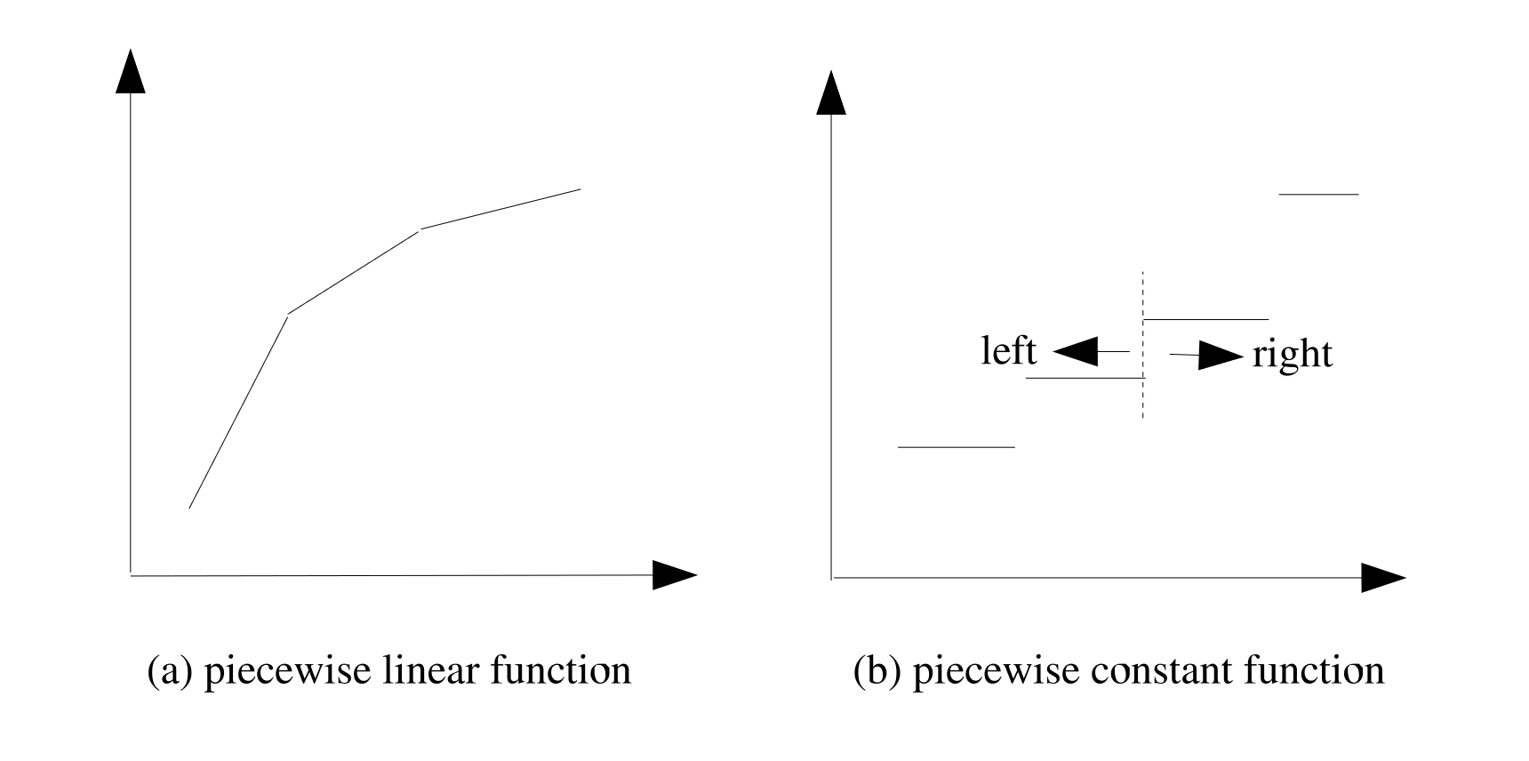
Fig. 2.1 Piecewise linear and piecewise constant functions.

• A PIECEWISE LINEAR function performs linear interpolations between the provided value pairs; a PIECEWISE CONSTANT function is constant valued between provided value pairs. Fig. 2.1 (a) shows an example of a piecewise linear function, and Fig. 2.1 (b) shows an example of a piecewise constant function.

• For functions that are based on tabular values, such as the PIECEWISE LINEAR and PIECEWISE CONSTANT functions, there is a possibility that the function may be evaluated for abscissa values that fall outside the range of the tabulated values. If the abscissa for which the function is to be evaluated is lower than the lowest tabulated abscissa, the function returns the ordinate corresponding to the smallest tabulated abscissa. Likewise, if the function is evaluated for an abscissa higher than the highest tabulated abscissa, the function returns the ordinate corresponding to the highest tabulated abscissa. For example, consider the following function:

  begin function my_func
    type = piecewise linear
    begin values
      5.0  0.0
      10.0 50000.0
    end values
  end function my_func
  

  For values less than 5, this function returns 0, and for values greater than 10, it returns 50000.

• PIECEWISE LINEAR and PIECEWISE CONSTANT functions must be defined with either monotonically increasing x-values (\(x_{i} >= x_{i-1}\)) or monotonically decreasing x-values (\(x_{i} <= x_{i-1}\)). For example, the following function definition is invalid:

  begin function my_func
    type = piecewise linear
    begin values
      0.0  0.0
      0.5  0.0
      1.0  1.0
      0.5  1.0
    end values
  end function my_func
  

• For a piecewise constant function, a constant valued segment ends on the left hand side of an abscissa value and a new constant value segment begins on the right hand side of the same abscissa value. (This transition from one constant value to another is indicated by the dotted line in Fig. 2.1 (b).) When the value of the function is to be evaluated at a discontinuity, where two potential values exist for the ordinate, the default behavior is to use the ordinate from the value pair that has the higher-valued abscissa. In other words, to use the value on the right hand side of the discontinuity. The AT DISCONTINUITY EVALUATE TO command line can be used to override this default behavior at an abscissa with two ordinate values. The command line can have a value of either LEFT or RIGHT. If RIGHT (the default) is specified, the ordinate value to the right of the abscissa is used; if LEFT is specified, the ordinate value to the left of the abscissa is used.

• The PIECEWISE MULTIVARIATE option allows the user to specify multiple independent variables and one dependent variable. The user specifies the names of these variables via the COLUMN TITLES line command. One must input the same number of column titles as there are columns in the function. The names input into the column titles must correspond to a field computed in Sierra/SM. The user must then provide the FIELD TYPES command line specifying the type of field they will be comparing in the function (e.g. GLOBAL, NODAL, or ELEMENT field). Example syntax is shown below:

  begin function multivariate_output
    type = piecewise multivariate
    column titles distance temperature displacement
    field types global nodal nodal
    begin values
      0.000   0.0    0.0
      0.002   0.0    0.0
      0.004   0.0    0.0
      0.000   10.0   1.0e-3
      0.002   10.0   2.0e-3
      0.004   10.0   3.0e-3
      0.000   20.0   5.0e-2
      0.002   20.0   10.0e-2
      0.004   20.0   15.0e-2
    end values
  end function
  

The PIECEWISE MULTIVARIATE option also has special use cases of being used with the Hydra Plasticity Material Model and the Persson Friction Model (Goodyear Specific). If the FIELD TYPES command is not specified, it will be assumed the user is running one of the two above use cases.

• The MULTICOLUMN PIECEWISE LINEAR function is not used in Sierra Solid Mechanics. It can be used in coupled analysis with Aria, Fuego, etc.

• The EVALUATE EXPRESSION command line consists of one or more user-supplied algebraic expressions. This command line must be used if the value on the TYPE command line is ANALYTIC. See the rules and options for composing algebraic expressions discussed below.

• The DIFFERENTIATE EXPRESSION command line consists of one or more user-supplied algebraic expressions. This command line must be used if the value on the TYPE command line is ANALYTIC and you need the derivative of the analytic function that you defined with EVALUATE EXPRESSION. This can happen if you are using an analytic function in a constitutive model. See the rules and options for composing algebraic expressions discussed below.

Importantly, a FUNCTION command block cannot contain both a VALUES command block and an EVALUATE EXPRESSION command line.

Rules and Options for Composing Algebraic Expressions. If you choose to use the EVALUATE EXPRESSION command line, you will need to write the algebraic expressions. The algebraic expressions are written using a C-like format. Each algebraic expression is terminated by a semicolon(;). The entire set of algebraic expressions, whether a single expression or several, is enclosed in a single set of double quotes(” “).

Note: analytic function variables are case insensitive, including any local variable definitions, and there is currently no warning for multiply-defined variables (the last variable name “wins”), so caution should be taken to ensure that duplicate variable names are not used.

Expressions compute an output value as a function of input values. The input value of an expression is called an independent variable of the expression. An expression can use any name for the expression independent variable. The examples shown here use x for the independent variable.

Example: Return sin(x) as the value of the function.

begin function sinx
  type is analytic
  evaluate expression is "sin(x)"
end

Example: Return a piecewise linear interpolated ramp function. For x values less than 0.0 the function will return 0.0. For x values between 0.0 and 0.5 the function will return y values linearly interpolated between 0 and 100. For x values greater than 0.5 the function will return 100:

begin function pressure
  type is analytic
  evaluate expression is "   \#
    (x <= 0.0) ? (           \#
      0.0                    \#
    ) : (                    \#
      (x < 0.5) ? (          \#
        x*200.0              \#
      ) : (                  \#
       100.0                 \#
      )                      \#
    )                        \#
   "
end

Operators and Functions Available within Expressions. The following functionality is currently implemented for the expressions:

• Operators Valid arithmetic and Boolean operations are as follows:

  Symbol	Operation
  +, -	plus, minus
  +, -	plus, minus
  *, /	times, divide
  ^	power
  ==, !=	equivalent, not equivalent
  >, <	greater/less than
  >=, <=	greater/less than or equal t
  !	not
  &, |, &&, ||	and, or
  ?, :	ternary if, then, else

• Parentheses (), represents standard mathematical meaning of operation ordering.

• Component indexing value[i], accesses the \(i\)th component of a multi-component variable such as a vector, tensor, etc. This index is one-based. For a vector vec,

  vec_x = vec[1]
  vec_y = vec[2]
  vec_z = vec[3]
  

  for a symmetric tensor sym,

  sym_xx = sym[1]
  sym_yy = sym[2]
  sym_zz = sym[3]
  sym_xy = sym[4]
  sym_yz = sym[5]
  sym_zx = sym[6]
  

  and for a full tensor full,

  full_xx = full[1]
  full_yy = full[2]
  full_zz = full[3]
  full_xy = full[4]
  full_yz = full[5]
  full_zx = full[6]
  full_yx = full[7]
  full_zy = full[8]
  full_xz = full[9]
  

• Math functions Valid mathematical operations are as follows:

  Function	Operation
  abs(x)	absolute value of x
  mod(x,y)	modulus of x``|``y
  min(x,y)	minimum value of x, y
  max(x,y)	maximum value of x, y
  sign(x)	sign operator: \(-1\) if x is negative, \(1\) if positive
  ipart(x)	integer part of x
  fpart(x)	fractional part of x

• Power functions Valid functions for expressions containing exponents are as follows:

  Function	Operation
  pow(x,y)	\(x^{y}\)
  pow10(x)	\(10^{x}\)
  sqrt(x)	\(\sqrt{x}\)

• Trigonometric functions Valid trigonometric operations are as follows:

  Function	Operation
  acos(x)	arccosine of x
  asin(x)	arcsine of x
  asinh(x)	inverse hyperbolic sin of x
  atan(x)	arctangent of x
  atan2(y,x)	arctangent of y/x, signs of x and y
  cos(x)	cosine of x
  cosh(x)	hyperbolic cosine of x
  sin(x)	sine of x
  sinh(x)	hyperbolic sine of x
  tan(x)	tangent of x
  tanh(x)	hyperbolic tangent of x

• Logarithm functions Valid logarithmic operations are as follows:

  Function	Operation
  log(x) or ln(x)	natural logarithm of x
  log10(x)	base-10 logarithm of x
  exp(x)	\(e^{x}\)

• Rounding functions Valid mathematical rounding operations are as follows:

  Function	Operation
  ceil(x)	smallest integer value not less than x
  floor(x)	largest integer value not greater than x

• Random functions Valid functions for generating random data are as follows:

  Function	Operation
  random()	random real number \(0.0 \le x < 1.0\)
  random(x)	seeds the random number generator
  time()	elapsed time in seconds since January 1, 1970

• Coordinate conversion functions Valid functions for converting to and from polar and Cartesian coordinate systems are as follows:

  Function	Operation
  deg(x)	converts x from radians to degrees
  rad(x)	converts x from degrees to radians
  recttopolr(x,y)	magnitude of vector (x, y)
  recttopola(x,y)	angle of vector (x, y)
  poltorectx(r,th)	\(x\)-coordinate of angle th at distance r
  poltorecty(r,th)	\(y\)-coordinate of angle th at distance r

• If, then, else ternary syntax A ? B : C, where A is a Boolean statement such as (x < 2.0), B is a statement (or set of statements) to be evaluated if A is true, and C is a statement (or set of statements) to be evaluated if A is false. Note: these statements can only be used for return values, i.e. you cannot define local variables inside a ternary statement.

• Other utilities Miscellaneous other utility functions are as follows:

  • cos_ramp(x, xstart, xend) defines a cosine ramp loading function. For x < xstart, it returns 0.0. For x > xend, it returns 1.0. If xstart <= x <= xend, the function has the value (1.0-cos(Pi*(x-xstart)/(xend-xstart)))/2.0. The primary purpose for the cosine ramp is to provide smooth loading. If attempting to run a nearly quasistatic problem with the dynamic solver, a displacement boundary condition applied via the cos_ramp will generally give a smooth response for a given loading time.

  • cycloidal_ramp(x, xstart, xend) defines a cycloidal ramp function. For x < xstart it returns 0.0. For x > xend, it returns 1.0. If xstart <= x <= xend, the function has the value (x-xstart)/(xend-xstart)-1/(2*pi)*sin(2*pi/(xend-xstart)*(x-xstart)). The primary purpose for the cycloidal front ramp is to provide smooth loading for prescribed displacements and velocities. This function has continuous acceleration derivatives at xstart and xend, providing a smoother response than the cos_ramp for prescribed displacement boundary conditions.

  • haversine_pulse(x, xstart, xend) defines a haversine pulse function. For x < xstart, it returns 0.0. For x > xend, it returns 0.0. If xstart <= x <= xend, the function has the value pow(sin(Pi*(x-xstart)/(xend-xstart)),2). Design shock loads for components are often specified as haversine acceleration pulses; this function is included to make it easier to apply this loading.

Constants. There are three predefined constants that may be used in an expression. These three constants are e, pi, and two_pi. Note that these constants are reserved variable names and thus cannot be redefined in an expression.

Math Symbol	Expression	Value
\(e\) e	\(2.7182818284\ldots\)
\(\pi\)	pi	\(3.1415926535\ldots\)
\(2\pi\)	two_pi	\(2*3.1415926535\ldots\)

Also, there are four predefined constant functions that can be used, SIERRA_CONSTANT_FUNCTION_ZERO, SIERRA_CONSTANT_FUNCTION_ONE, SIERRA_LINEAR_RAMP_FUNCTION, and SIERRA_COS_RAMP_FUNCTION. The first two functions are equivalent to defining functions with constant expressions “0.0” or “1.0”, respectively. The third function is the equivalent to a linear ramp in time with a slope of 1.0, and the fourth function is identical to a cos_ramp that ramps from 0.0 at the start time of the simulation to 1.0 at the termination time. See Appendix A for a full list of pre-defined options that can be used in an input deck.

The PIECEWISE ANALYTIC function is a combination of several analytic functions that are evaluated over different ranges of x. As an example consider the following function. The function ramps up a load from time 0.0 to 1.0, holds that load constant from time 1.0 to 2.0, ramps the load back down to zero from time 2.0 to 3.0, and then holds the load constant again after time 3.0.

begin function force_ramp
  type is piecewise analytic
  begin expressions
    0.0 "(1.0-cos(pi*x))/2.0"
    1.0 "1.0"
    2.0 "(1.0+cos(pi*(x-2.0)))/2.0"
    3.0 "0.0"
  end
end

Note this function is equivalent to the single compound, ANALYTIC function below, though the piecewise version tends to be easier to read. The expression compound if then else statement below also demonstrates the recommended indentation for nested if statements. The statement could be written on a single line, but the indentation makes the logic of the evaluation statement more readable.

begin function force_ramp
  type is analytic
  evaluate expression = "            \#
    (x < 1.0) ? (                    \#
      (1.0-cos(pi*x))/2.0            \#
    ) : (                            \#
      (x < 2.0) ? (                  \#
        1.0                          \#
      ) : (                          \#
        (x < 3.0) ? (                \#
          (1.0+cos(pi*(x-2.0)))/2.0  \#
        ) : (                        \#
          0.0                        \#
        )                            \#
      )                              \#
    )                                \#
  "
end

2.1.6. General Functions

BEGIN FUNCTION <string>function_name
  TYPE = ANALYTIC|PIECEWISE ANALYTIC

  EXPRESSION VARIABLE: <var_name> = NODAL|NODAL_VECTOR|
     NODAL_TENSOR|NODAL_SYM_TENSOR|ELEMENT|ELEMENT_VECTOR|
     ELEMENT_TENSOR|ELEMENT_SYM_TENSOR|FACE|GLOBAL <var_source>

  BEGIN EXPRESSIONS
    <real>x_1   <string>analytic_expression_1
    <real>x_2   <string>analytic_expression_2
    ...
    <real>x_n   <string>analytic_expression_n
  END
  AT DISCONTINUITY EVALUATE TO <string>LEFT|RIGHT(LEFT)
  EVALUATE EXPRESSION = <string>analytic_expression1;
    analytic_expression2; ...
END [FUNCTION <string>function_name]

General functions can compute a global, element, or nodal scalar value that is a function of several input values. Each input value to the function is explicitly defined via an EXPRESSION VARIABLE command. The expression variable command defines variable for use in an expression or expression list. As an example consider a function to apply a combination of shearing and extension to a block. An example displacement map going from time zero to time one is shown in Fig. 2.2. The equation for this displacement map is given by:

\[\Delta_x(x,y,t) = t * (0.5 * x + 0.5 * y)\]

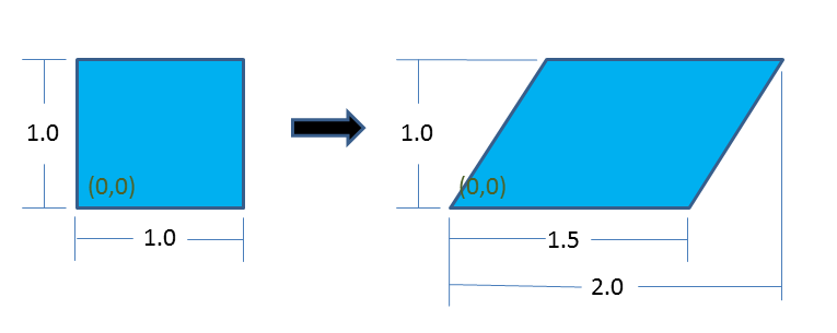
Fig. 2.2 Example displacement map.

This displacement map can be applied by a combination of a general function and a displacement boundary condition by:

BEGIN FUNCTION delta_x
  TYPE = analytic
  EXPRESSION variable: mx   = NODAL model_coordinates(x)
  EXPRESSION variable: my   = NODAL model_coordinates(y)
  EXPRESSION variable: time = GLOBAL time
  EVALUATE EXPRESSION = "time * (0.5*mx + 0.5*my)"
END

BEGIN PRESCRIBED DISPLACEMENT
  BLOCK = BLOCK_1
  COMPONENT = X
  FUNCTION = delta_x
END

The model_coordinates are the initial nodal coordinates. Time is the current analysis time. If a general function is being applied to a nodal boundary condition, such as displacement, function will be evaluated at each node. On a node the value of model_coordinates will be extracted and placed into the expression variables mx and my. The analysis time is placed into the expression variable time. The expression is then evaluated producing a single value at the node, the nodal value is used to define the x displacement at that particular node.

A function used to define nodal quantities may reference NODAL or GLOBAL expression variables. A function used to define an element quantity may reference ELEMENT or GLOBAL expression variables. A function used to define a global quantity may only reference GLOBAL expression variables. Generally any quantity that would be available for output at nodes, at elements, or as a global variable may be used as an expression variable.

Expression variables may also accept vectors, tensors or symmetric tensors. A vector can define variables in terms of x, y, and z. For example,

EXPRESSION variable: A = element_vector velocity

would define A_x, A_y, and A_z for use in an expression. A symmetric tensor can define variables in terms of xx, yy, zz, zy, yz, and zx. For example,

EXPRESSION variable: A = element_sym_tensor unrotated_stress

would define A_xx, A_yy, A_zz, A_xy, A_yz, and A_zx for use in an expression. A tensor can define variables in terms of xx, yy, zz, zy, yz, zx, yz, xz, and zy.

EXPRESSION variable: A = element_tensor rotation

would define A_xx, A_yy, A_zz, A_xy, A_yz, A_zx, A_yx, A_zy, and A_xz. Particularly for tensors, this provides a clearer syntax for accessing the components of a multi-component variable.

Example of use:

# Define using named vector components
BEGIN FUNCTION velocity_vec
  TYPE = analytic
  EXPRESSION variable: V = nodal_vector velocity
  EVALUATE EXPRESSION = "sqrt((V_x)^2 + (V_y)^2 + (V_z)^2 )"
END

# Equivalent function using general variable indexing
BEGIN FUNCTION velocity_index
  TYPE = analytic
  EXPRESSION variable: V = nodal velocity
  EVALUATE EXPRESSION = "sqrt(V[1]^2 + V[2]^2 + V[3]^2 )"
END

...

BEGIN USER OUTPUT
  # speed1 and speed2 are equivalent, both are a nodal field that
  # is the local magnitude of the nodal velocity field
  compute nodal speed1 as function velocity_vec
  compute nodal speed2 as function velocity_index
END

2.1.7. Axes, Directions, and Points

DEFINE POINT <string>point_name WITH COORDINATES
  <real>value_1 <real>value_2 <real>value_3
DEFINE DIRECTION <string>direction_name WITH VECTOR
  <real>value_1 <real>value_2 <real>value_3
DEFINE AXIS <string>axis_name WITH POINT
  <string>point_1 POINT <string>point_2
DEFINE AXIS <string>axis_name WITH POINT
  <string>point DIRECTION <string>direction

Many Sierra/SM features require the definition of geometric entities. For instance, the prescribed displacement boundary condition requires a direction definition, and the cylindrical velocity initial condition requires an axis definition. Currently, Sierra/SM input permits the definition of points, directions, and axes. Definition of these geometric entities occurs in the SIERRA scope.

The DEFINE POINT command line is used to define a point:

DEFINE POINT <string>point_name WITH COORDINATES
  <real>value_1 <real>value_2 <real>value_3

where

• The string point_name is a name for this point. This name must be unique to all other points defined in the input file.

• The real values value_1, value_2, and value_3 are the \(x\), \(y\), and \(z\) coordinates of the point.

The predefined point SIERRA_POINT_ORIGIN can be used to specify a point at the origin of the global coordinate system. Refer to Appendix A for a full list of predefined options that can be used in an input deck.

The DEFINE DIRECTION command line is used to define a direction:

DEFINE DIRECTION <string>direction_name WITH VECTOR
  <real>value_1 <real>value_2 <real>value_3

where

• The string direction_name is a name for this direction. This name must be unique to all other directions defined in the input file.

• The real values value_1, value_2, and value_3 are the \(x\), \(y\), and \(z\) magnitudes of the direction vector.

The predefined directions SIERRA_DIRECTION_X, SIERRA_DIRECTION_Y, SIERRA_DIRECTION_Z, SIERRA_DIRECTION_NEG_X, SIERRA_DIRECTION_NEG_Y, and SIERRA_DIRECTION_NEG_Z can be used to specify the global axis directions +x, +y, +z, -x, -y, and -z, respectively. Refer to Appendix A} for a full list of predefined options that can be used in an input deck.

There are two command lines that can be used to define an axis. The first DEFINE AXIS command line uses two points:

DEFINE AXIS <string>axis_name WITH POINT
  <string>point_1 POINT <string>point_2

where

• The string axis_name is a name for this axis. This name must be unique to all other axes defined in the input file.

• The strings point_1 and point_2 are the names for two points defined in the input file via a DEFINE POINT command line.

The second DEFINE AXIS command line uses a point and a direction:

DEFINE AXIS <string>axis_name WITH POINT
  <string>point DIRECTION <string>direction

where

• The string axis_name is a name for this axis. This name must be unique to all other axes defined in the input file.

• The string point is the name of a point defined in the input file via a DEFINE POINT command line.

• The string direction is the name of a direction defined in the input file via a DEFINE DIRECTION command line.

2.1.8. Orientation

BEGIN ORIENTATION <string>orientation_name
  SYSTEM = <string>RECTANGULAR|Z_RECTANGULAR|CYLINDRICAL|
    SPHERICAL(RECTANGULAR)
  #
  POINT A = <real>global_ax <real>global_ay <real>global_az
  POINT B = <real>global_bx <real>global_by <real>global_bz
  #
  ROTATION ABOUT <integer> 1|2|3(2) = <real>theta(0.0)
END [ORIENTATION <string>orientation_name]

The ORIENTATION command block is currently used in Sierra/SM to define a local co-rotational coordinate system at each shell element centroid for output of shell in-plane stresses and strains. Each BEGIN SHELL SECTION command block has an orientation that generates this local coordinate system for each element in the associated element blocks. The generated local coordinate system rotates with the shell element, thus making it co-rotational.

Stresses and strains for shell elements are computed in the shell element’s local coordinate system, which typically varies from one element to the next, and can be seen in Fig. 2.3. The local \(\mathbf{R}\) axis of element 1 does not align with the local \(\mathbf{R}\) axis of element 2. Thus without the use of an orientation to rotate the local coordinate system in to a consistent coordinate system, stress and strain results would be difficult to decipher. The use of an orientation generates a transformation matrix from a shell element’s local \(\mathbf{R}\), \(\mathbf{S}\), \(\mathbf{T}\) coordinate system to the final coordinate system, \(\mathbf{R}'\), \(\mathbf{S}'\), \(\mathbf{T}'\), by use of orientation and element-specific basis vectors and a rotation about an axis, all defined below.

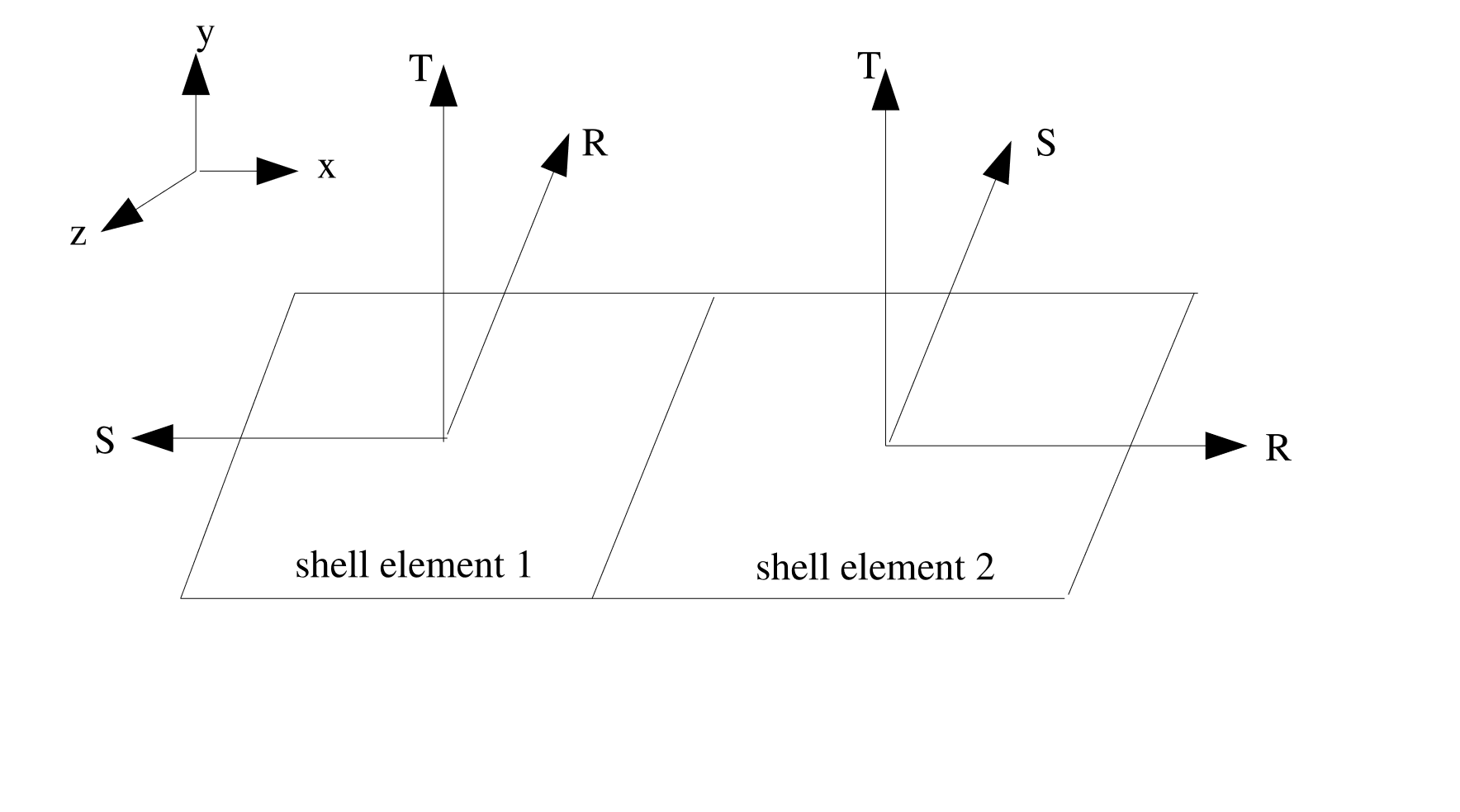
Fig. 2.3 Adjacent shell elements with non-aligned local coordinate systems.

There are four orientation systems available in Sierra/SM to better align the stress and strain output of shell elements. These orientations are defined via the optional SYSTEM command line within the ORIENTATION command block and are: RECTANGULAR, Z_RECTANGULAR, CYLINDRICAL and SPHERICAL with the default being RECTANGULAR. If the ORIENTATION command line within a SHELL SECTION block is not used, the default orientation is a RECTANGULAR system with axes aligned with the global X,Y and Z axes.

Each of the four systems produces a unique set of bases vectors, \(\mathbf{g}_1,\mathbf{g}_2,\mathbf{g}_3\), computed using the centroid of the shell element and the two required inputs, POINT A and POINT B. These four methods of computing \(\mathbf{g}_1,\mathbf{g}_2,\mathbf{g}_3\) are described below.

• RECTANGULAR: POINT A defines a point, \(P_A\), in the local coordinate system of the shell element that lies in the direction of the first basis vector, \(\mathbf{g}_1\), from the centroid, \(C\) with local coordinate of \((0,0,0)\), see Fig. 2.4. Thus, the vector from the centroid of the element to point \(P_A\) is defined as \(\mathbf{p}_A = P_A - C\). Similarly, a vector from the centroid to point \(P_B\), defined via POINT B, can be computed as \(\mathbf{p}_B = P_B - C\). Using these two vectors, the rectangular basis vectors are defined as: \(\mathbf{g}_1 = \frac{\mathbf{p}_A}{\parallel \mathbf{p}_A \parallel}\), \(\mathbf{g}_3 = \frac{\mathbf{g}_1 \times \mathbf{p}_B}{\parallel \mathbf{g}_1 \times \mathbf{p}_B \parallel}\), \(\mathbf{g}_2 = \frac{\mathbf{g}_3 \times \mathbf{g}_1}{\parallel \mathbf{g}_3 \times \mathbf{g}_1 \parallel}\).

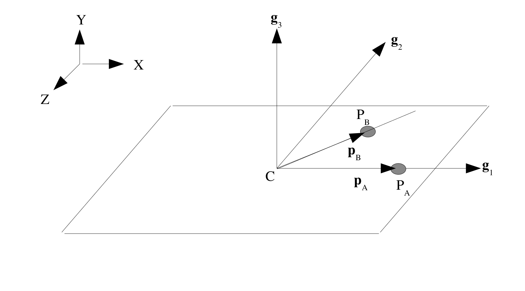
Fig. 2.4 Rectangular coordinate system.

• Z_RECTANGULAR: This set of basis vectors is defined similarly to the RECTANGULAR system, however point \(P_A\) now defines a point that lies in the direction of the third basis vector, \(\mathbf{g}_3\) from the centroid of the element, see Fig. 2.5. Using the same definition for \(\mathbf{p}_A\) and \(\mathbf{p}_B\) as above we can define the three basis vectors as: \(\mathbf{g}_3 = \frac{\mathbf{p}_A}{\parallel \mathbf{p}_A \parallel}\), \(\mathbf{g}_2 = \frac{\mathbf{g}_3 \times \mathbf{p}_B}{\parallel \mathbf{g}_3 \times \mathbf{p}_B \parallel}\), \(\mathbf{g}_1 = \frac{\mathbf{g}_2 \times \mathbf{g}_3}{\parallel \mathbf{g}_2 \times \mathbf{g}_3 \parallel}\).

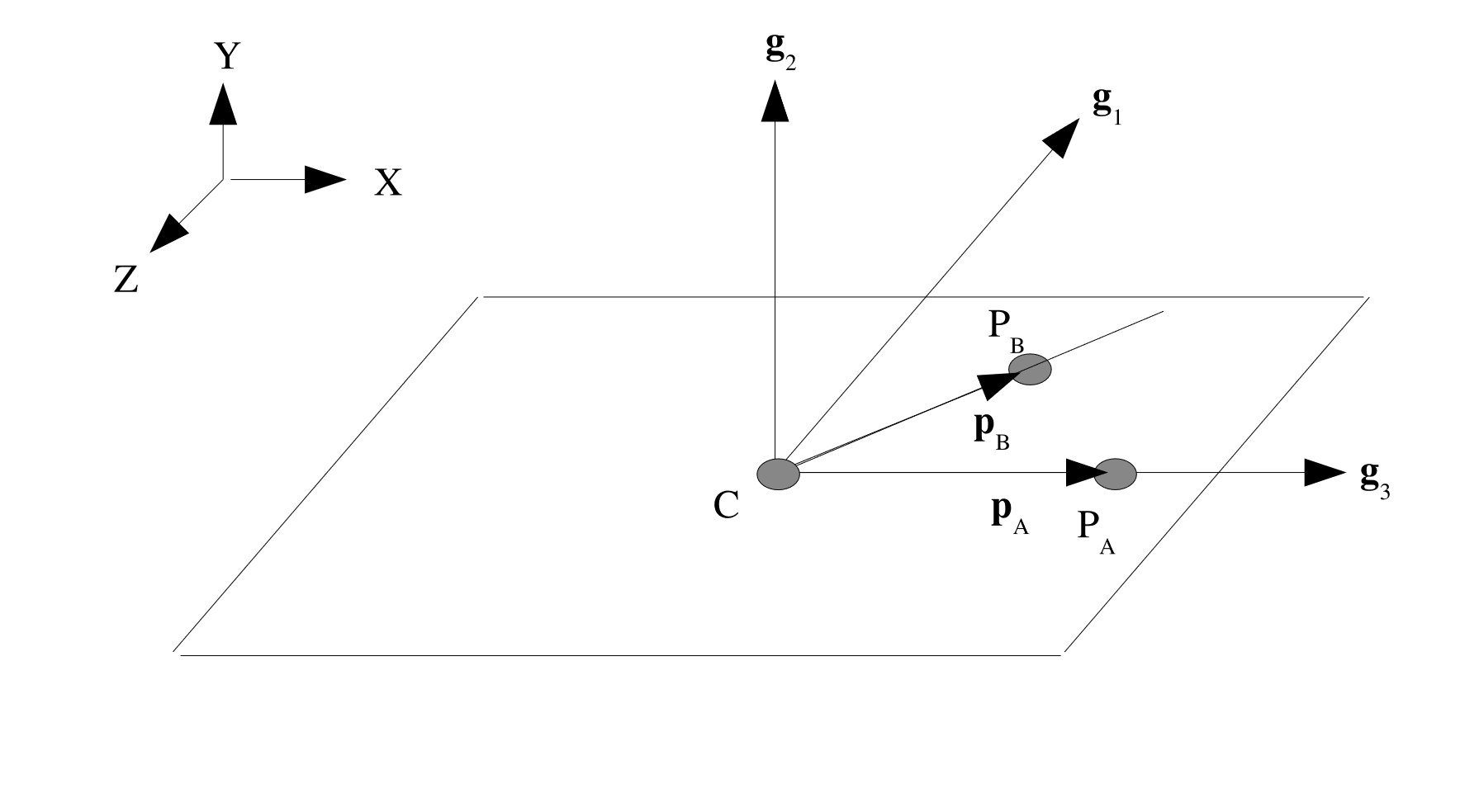
Fig. 2.5 Z-Rectangular coordinate system.

• CYLINDRICAL: POINT A, \(P_A\), and POINT B, \(P_B\), define the direction of the third basis vector, \(\mathbf{g}_3\) such that \(\mathbf{g}_3 = \frac{P_B - P_A}{\parallel P_B - P_A \parallel}\), as seen in Fig. 2.6. Defining a vector, \(\mathbf{v}\), from \(P_A\) to the centroid of the element, \(C\) in the global coordinate system, the second basis vector, \(\mathbf{g}_2\) is defined as: \(\mathbf{g}_2 = \frac{\mathbf{v} \times \mathbf{g}_3}{\parallel \mathbf{v} \times \mathbf{g}_3 \parallel}\). Therefore the first basis vector is defined as \(\mathbf{g}_1 = \frac{\mathbf{g}_2 \times \mathbf{g}_3}{\parallel \mathbf{g}_2 \times \mathbf{g}_3 \parallel}\).

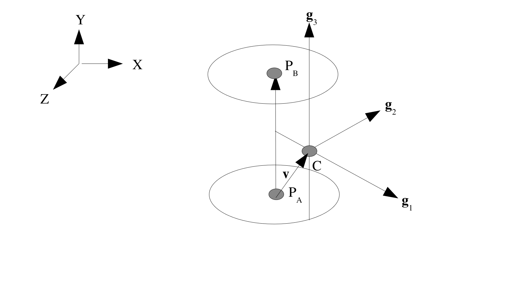
Fig. 2.6 Cylindrical coordinate system.

• SPHERICAL: The point \(P_A\), from the POINT A command line, defines the center of a sphere. The point \(P_B\), from the POINT B command line, defines a polar axis for the sphere. (See Fig. 2.7.) The first basis vector is defined by the vector that passes from \(P_A\) to the centroid, \(C\) in the global coordinate system, of the element: \(\mathbf{g}_1 = \frac{C - P_A}{\parallel C - P_A \parallel}\). The third basis vector is parallel to the vector from \(P_A\) to \(P_B\) such that \(\mathbf{g}_3 = \frac{P_B - P_A}{\parallel P_B - P_A \parallel}\). From these two vector, the second basis vector is defined as \(\mathbf{g}_2 = \frac{\mathbf{g}_3 \times \mathbf{g}_1}{\parallel \mathbf{g}_3 \times \mathbf{g}_1 \parallel}\). If \(\mathbf{g}_1\) and \(\mathbf{g}_3\) are collinear, the second basis vector is taken to be the normal of the element, \(\mathbf{T}\), and the third basis is \(\mathbf{g}_3 = \frac{\mathbf{g}_1 \times \mathbf{g}_2}{\parallel \mathbf{g}_1 \times \mathbf{g}_2 \parallel}\).

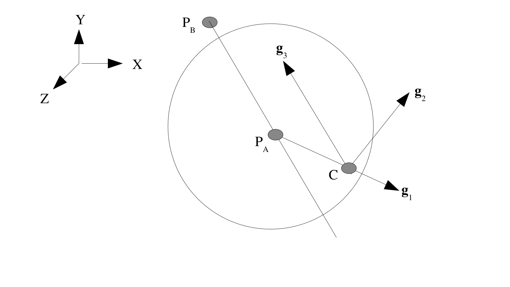
Fig. 2.7 Spherical coordinate system.

It is possible, using the ROTATION ABOUT command line, to specify an angle and an axis to rotate the basis vectors, \(\mathbf{g}_1\), \(\mathbf{g}_2\) and \(\mathbf{g}_3\) about to produce a second set of basis vectors, \(\mathbf{g}'_1\), \(\mathbf{g}'_2\) and \(\mathbf{g}'_3\), that are then used to compute the final transformation matrix. The syntax for this command is as follows:

ROTATION ABOUT 1|2|3(2) = <real>theta(0.0)

Where the 1,2,3 refers to which basis vector the rotation will occur about. The default value is 2 with an angle theta of 0.0, thus implying a rotation of 0.0 radians about \(\mathbf{g}_2\). How \(\mathbf{g}'_1\), \(\mathbf{g}'_2\) and \(\mathbf{g}'_3\) are computed for each of the three cases is described below. In each case, the second order rotation tensor, \(\mathbf{Q}\), is defined as:

\[\begin{split}\mathbf{Q} = \left[\begin{array}{ccc} 2(q_0^2 + q_1^2) - 1 & 2(q_1 q_2 - q_0q_3) & 2(q_1 q_3 - q_0 q_3) \\ 2(q_1 q_2 + q_0 q_3) & 2(q_o^2 + q_2^2) - 1 & 2(q_2 q_3 - q_0 q_1) \\ 2(q_1 q_3 - q_0 q_2) & 2(q_2 q_3 + q_0 q_1) & 2(q_0^2 + q_3^2) - 1 \end{array}\right]\end{split}\]

Where: \(q_0 = \cos(\frac{\theta}{2})\), \(q_1 = a_1 \sin(\frac{\theta}{2})\), \(q_2 = a_2 \sin(\frac{\theta}{2})\), and \(q_3 = a_3 \sin(\frac{\theta}{2})\), where the vector \(\mathbf{a} = [a_1, a_2, a_3]\) is the basis vector we are rotating about.

• Rotation about \(\mathbf{g}_1\) (ROTATION ABOUT 1): The prime set of basis vectors are defined as: \(\mathbf{g}'_1 = \mathbf{Q}\mathbf{g}_3\), \(\mathbf{g}'_2 = \mathbf{Q}\mathbf{g}_2\), \(\mathbf{g}'_3 = -\mathbf{g}_1\). Which can graphically be seen in Fig. 2.8.

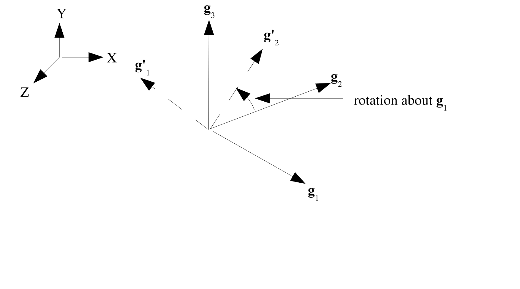
Fig. 2.8 Rotation about 1.

• Rotation about \(\mathbf{g}_2\) (ROTATION ABOUT 2), default: The prime set of basis vectors are defined as: \(\mathbf{g}'_1 = \mathbf{Q}\mathbf{g}_1\), \(\mathbf{g}'_2 = \mathbf{Q}\mathbf{g}_3\), \(\mathbf{g}'_3 = -\mathbf{g}_2\).

• Rotation about \(\mathbf{g}_3\) (ROTATION ABOUT 3): The prime set of basis vectors are defined as: \(\mathbf{g}'_1 = \mathbf{Q}\mathbf{g}_2\), \(\mathbf{g}'_2 = \mathbf{Q}\mathbf{g}_1\), \(\mathbf{g}'_3 = -\mathbf{g}_3\).

The next step is to project \(\mathbf{g}'_1\) onto the shell face as follows: \(\mathbf{R}' = \mathbf{g}'_1 - (\mathbf{g}'_1 \cdot \mathbf{T}) \mathbf{T}\), which defines a rotated \(\mathbf{R}\) vector. If \(\mathbf{R}'\) is perpendicular to the face of the element, we then redefine \(\mathbf{R}'\) to be: \(\mathbf{R}' = \mathbf{g}'_2 - (\mathbf{g}'_2 \cdot \mathbf{T}) \mathbf{T}\), the projection of \(\mathbf{g}'_2\) onto the element face. Once we have \(\mathbf{R}'\) we can define \(\mathbf{S}'\) as \(\frac{\mathbf{T} \times \mathbf{R}'}{\parallel \mathbf{T} \times \mathbf{R}' \parallel}\). Hence, the final transformation matrix taking local stress and strain (in the \(\mathbf{R}\), \(\mathbf{S}\) coordinate system) to the \(\mathbf{R}'\), \(\mathbf{S}'\) coordinate system is:

\[\begin{split}\mathbf{Q}' = \left[\begin{array}{ccc} \mathbf{R} \cdot \mathbf{R}' & \mathbf{R} \cdot \mathbf{S}' & 0 \\ \mathbf{S} \cdot \mathbf{R}' & \mathbf{S} \cdot \mathbf{S}' & 0 \\ 0 & 0 & 1 \end{array}\right]\end{split}\]

2.1.9. Coordinate System Block Command

The RECTANGULAR|CYLINDRICAL|SPHERICAL|CONICAL|ELLIPSOIDAL|TOROIDAL COORDINATE SYSTEM command block is used to define a local coordinate system for transforming a stress tensor from components in the global \(x,y,z\) coordinate system to the local system for output.

This command block cannot be used for in-plane stresses and strains of shell elements because the shell integration point stresses and strains are computed in a local element system that varies element to element and rotates with the element. For output of shell stresses, the BEGIN ORIENTATION command must be used as explained in Section 2.1.8.

The COORDINATE SYSTEM block is also used to define a local coordinate system on the elements of a block for use in a representative volume analysis. In these analyses, elements of each representative volume will be aligned with the local system defined on the parent element.

BEGIN RECTANGULAR COORDINATE SYSTEM <string>name
  ORIGIN = <real> <real> <real>
  Z POINT = <real> <real> <real>  # Point on Z-tilde axis
  XZ POINT = <real> <real> <real> # Point on X-tilde-Z-tilde plane
END

BEGIN RECTANGULAR COORDINATE SYSTEM <string>name
  ORIGIN NODESET  = <nodelist>    # Single-node nodesets
  Z POINT NODESET  = <nodelist>   # Node on Z-tilde axis
  XZ POINT NODESET = <nodelist>   # Node on X-tilde-Z-tilde plane
END

BEGIN CYLINDRICAL COORDINATE SYSTEM <string>name
  ORIGIN = <real> <real> <real>
  Z POINT = <real> <real> <real>  # Point on Z-tilde axis
  XZ POINT = <real> <real> <real> # Optional: point on X-tilde-Z-tilde plane; sets
                                  # location of azimuthal angle theta=0
END

BEGIN CYLINDRICAL COORDINATE SYSTEM <string>name
  ORIGIN NODESET  = <nodelist>    # Single-node nodesets
  Z POINT NODESET  = <nodelist>   # Node on Z-tilde axis
  XZ POINT NODESET = <nodelist>   # Optional: node on X-tilde-Z-tilde plane; sets
                                  # location of azimuthal angle theta=0
END

BEGIN SPHERICAL COORDINATE SYSTEM <string>name
  ORIGIN = <real> <real> <real>
  Z POINT = <real> <real> <real>  # Point on Z-tilde axis
  XZ POINT = <real> <real> <real> # Optional: point on X-tilde-Z-tilde plane; sets
                                  # location of azimuthal angle theta=0
END

BEGIN SPHERICAL COORDINATE SYSTEM <string>name
  ORIGIN NODESET  = <nodelist>    # Single-node nodesets
  Z POINT NODESET  = <nodelist>   # Node on Z-tilde axis
  XZ POINT NODESET = <nodelist>   # Optional: node on X-tilde-Z-tilde plane; sets
                                  # location of azimuthal angle theta=0
END

BEGIN CONICAL COORDINATE SYSTEM <string>name
  ORIGIN = <real> <real> <real>
  Z POINT = <real> <real> <real>  # Point on Z-tilde axis
  XZ POINT = <real> <real> <real> # Optional: point on X-tilde-Z-tilde plane
  ANGLE = <real>
END

BEGIN CONICAL COORDINATE SYSTEM <string>name
  ORIGIN NODESET  = <nodelist>    # Single-node nodesets
  Z POINT NODESET  = <nodelist>   # Node on Z-tilde axis
  XZ POINT NODESET = <nodelist>   # Optional: Node on X-tilde-Z-tilde plane
  ANGLE = <real>
END

BEGIN ELLIPSOIDAL COORDINATE SYSTEM <string>name
  ORIGIN = <real> <real> <real>
  Z POINT = <real> <real> <real>  # Point on Z-tilde axis
  XZ POINT = <real> <real> <real> # Point on X-tilde-Z-tilde plane
  AXIS STRETCHING = <real> <real> <real> #angle in radians
END

BEGIN ELLIPSOIDAL COORDINATE SYSTEM <string>name
  ORIGIN NODESET  = <nodelist>    # Single node nodeset
  Z POINT NODESET  = <nodelist>
  XZ POINT NODESET = <nodelist>
  AXIS STRETCHING = <real> <real> <real> #angle in radians
END

BEGIN TOROIDAL COORDINATE SYSTEM <string>name
  ORIGIN = <real> <real> <real>
  Z POINT = <real> <real> <real>  # Point on Z-tilde axis
  XZ POINT = <real> <real> <real> # Point on X-tilde-Z-tilde plane
  MAJOR RADIUS = <real> #Toroid radius
END

BEGIN TOROIDAL COORDINATE SYSTEM <string>name
  ORIGIN NODESET  = <nodelist>    # Single node nodeset
  Z POINT NODESET  = <nodelist>
  XZ POINT NODESET = <nodelist>
  MAJOR RADIUS = <real> #Toroid radius
END

The prefix to COORDINATE SYSTEM specifies the type of local coordinate system. Supported types are: RECTANGULAR (Cartesian), CYLINDRICAL (Polar), SPHERICAL, CONICAL (a cylindrical system with an aperture angle), ELLIPSOIDAL (a spherical system stretched by AXIS STRETCHING), and TOROIDAL (a coordinate system aligned with a torus.)

A local element coordinate system is defined by a set of three control points. These points may be defined using absolute locations (ORIGIN, Z POINT, XZ POINT) or using nodelists in the mesh file (ORIGIN NODESET, Z POINT NODESET, XZ POINT NODESET) that contain exactly one node each. The control points define a local \(\tilde{X}\,\tilde{Y}\,\tilde{Z}\) Cartesian coordinate system centered at the coordinate system origin. For cylindrical, spherical, conical, ellipsoidal, and toroidal systems the orientation of the basis vectors at individual nodes and elements is spatially dependent. In this documentation, the local basis vectors at each node or element will be denoted as \(\hat{r}\) \(\hat{s}\) and \(\hat{t}\)

NOTE: When using nodesets instead of points, the defined coordinate system will be dynamic and will translate and rotate.

• ORIGIN: Required. Specifies the origin location for the new coordinate system. Replace with ORIGIN NODESET for a dynamic system.

• Z POINT: Required. Specifies a point on the \(\tilde{Z}\) axis for the new coordinate system. Replace with Z POINT NODESET for a dynamic system. For SPHERICAL, this defines where the zenith (polar) angle \(\phi\) is 0.

• XZ POINT: Required only for RECTANGULAR and ELLIPSOIDAL. Third point to specify the \(\tilde{X}\tilde{Z}\)-plane of the new system. Must not lie on the \(\tilde{Z}\) axis. If not specified, an arbitrary axis will be chosen based on the global coordinate system. Replace with XZ POINT NODESET for a dynamic system. For CYLINDRICAL and SPHERICAL, this defines where the azimuthal angle \(\theta\) is 0. XZ POINT also affects behavior at ill-defined points such as the origin of SPHERICAL systems, or along the \(\tilde{Z}\) axis of CYLINDRICAL systems (see Fig. 2.14).

• ANGLE (CONICAL COORDINATE SYSTEM only): Required. Defines the angle in radians to rotate the axial direction away from the \(\tilde{Z}\) axis (see Fig. 2.11).

• AXIS STRETCHING (ELLIPSOIDAL COORDINATE SYSTEM only): Required. Defines the aspect ratio to stretch a spherical system (see Fig. 2.12).

• MAJOR RADIUS (TOROIDAL COORDINATE SYSTEM only): Required. Defines the torus major radius (see Fig. 2.13).

The three coordinate control points are illustrated in Fig. 2.9. The coordinate system types are depicted in Fig. 2.11, Fig. 2.12, Fig. 2.13, and Fig. 2.10.

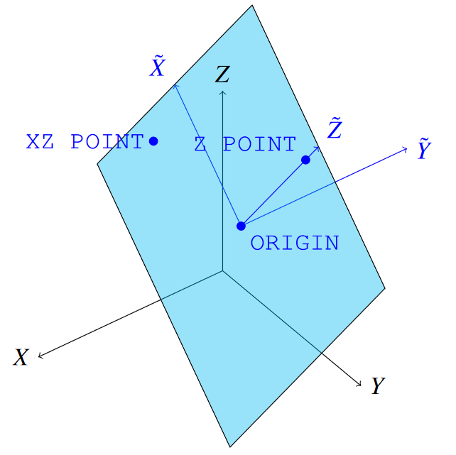
Fig. 2.9 Coordinate system definition vectors: note that XZ POINT determines the \(\tilde{X}\) axis, but need not lie along it, which is the case depicted in this figure.

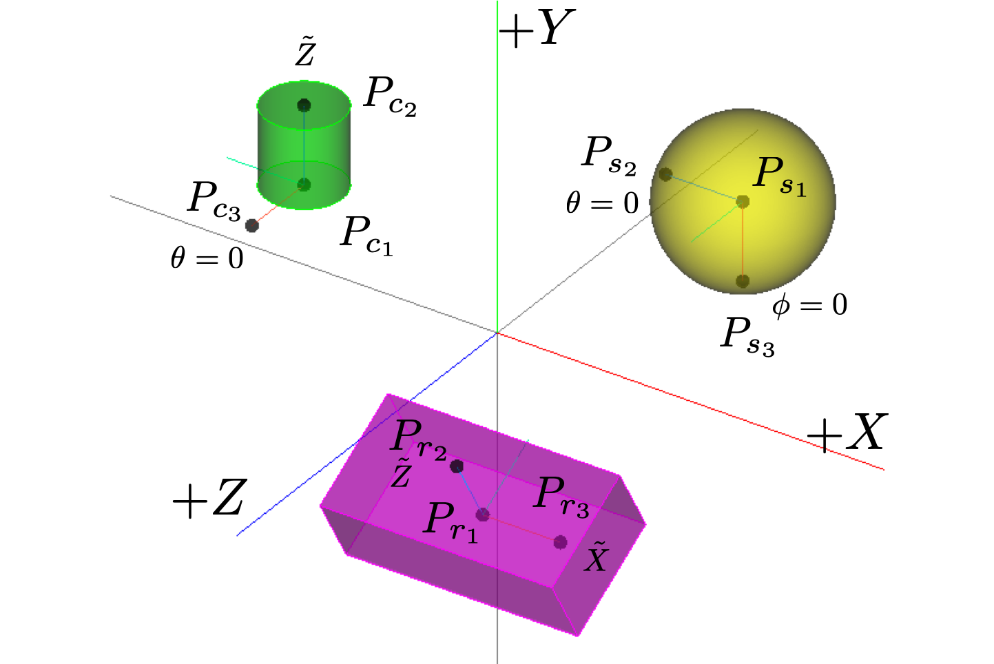
Fig. 2.10 Three examples (rectangular, spherical, and cylindrical) of transformed coordinate systems are given. The center of the rectangular block \((6\times2\times3)\) is located at \((3, -1, 5)\), and rotated 30 degrees about the \(X\) axis. The center of the sphere (radius of 2) is located at \((5, 4, -2)\). The center of the cylinder (radius of 1, height of 2, and rotated 90 degrees about the \(X\) axis) is located at \((-5, 2, 0)\). The new coordinate systems are defined respectively of each of the geometries, and are indicated by \(\tilde{X}\,\tilde{Y}\,\tilde{Z}\) and the subscripts (\(r\), \(s\), and \(c\)).

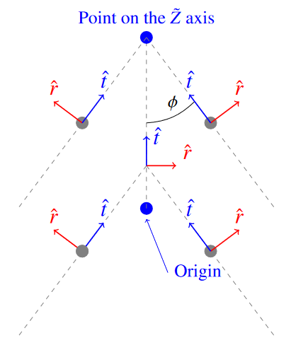
Fig. 2.11 Conical Coordinate System Definition at \(\tilde{X}\tilde{Z}\) plane.

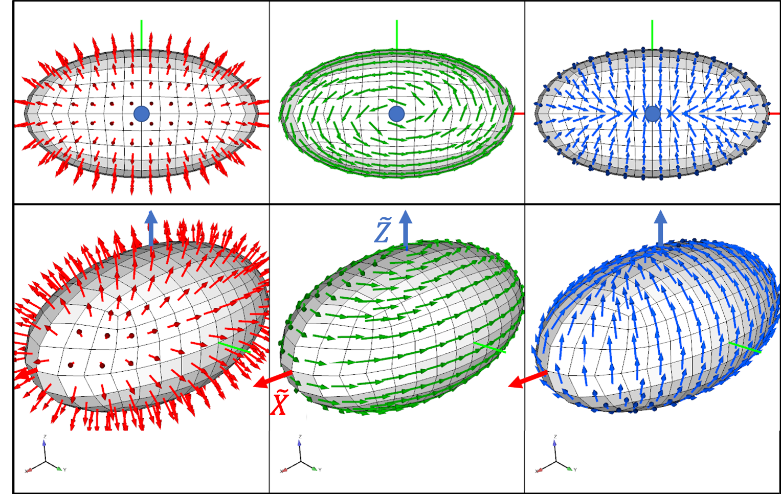
Fig. 2.12 Ellipsoidal Coordinate System Using axis_stretching=(2.0, 1.1, 1.0). \(\hat{r}\) is red, \(\hat{s}\) is green, and \(\hat{t}\) is blue.

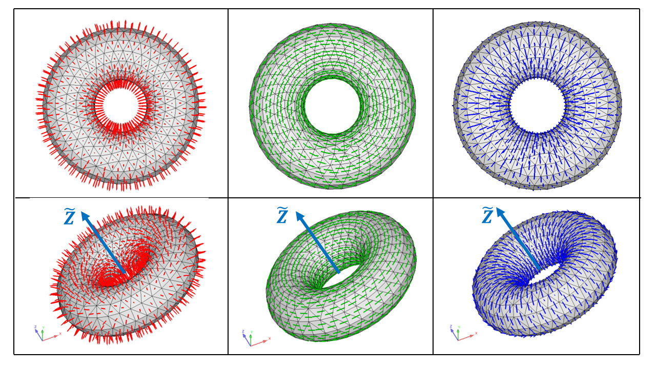
Fig. 2.13 Toroidal Coordinate System Using major_radius=(2.0). \(\hat{r}\) is red, \(\hat{s}\) is green, and \(\hat{t}\) is blue.

Examples of rectangular, spherical, and cylindrical coordinate systems are given in Fig. 2.10. In those examples, we wish to define coordinate systems for three geometries: a brick, a sphere, and cylinder. The corresponding input deck is shown below.

begin rectangular coordinate system rectangular_system
  origin   3 -1 5
  z point  5 -1 5
  xz point 3 0.7321 6
end
coordinate spherical coordinate system ball_like
  origin 5 4 -2
  z point 5 2 -2
  xz point 3 4 -2
end
begin cylindrical coordinate pin_system
  origin -5 2 0
  z point -5 4 0
  xz point -5 2 2
end

For cylindrical, conical, spherical, ellipsoidal, and toroidal systems, the local basis vectors \(\hat{r}\), \(\hat{s}\), and \(\hat{t}\) are not all well-defined when sampled along the \(\tilde{Z}\) axis. At the origin, all coordinate systems fall back to a local Cartesian system with \(\hat{r}\) along the \(\tilde{X}\) axis, \(\hat{s}\) along the \(\tilde{Y}\) axis, and \(\hat{t}\) along the \(\tilde{Z}\) axis. This is also true for the cylindrical and conical systems on the \(\tilde{Z}\) axis. Spherical and ellipsoidal systems on the \(\tilde{Z}\) axis will instead maintain the first vector (\(\hat{r}\)) pointing radially outward, the third vector (\(\hat{t}\)) pointing along the \(\tilde{X}\) axis, and the second vector (\(\hat{s}\)) as either the positive or negative \(\tilde{Y}\) axis (generating a right handed system). This maintains the normal and tangential properties of the three vectors for spherical coordinates. See Fig. 2.14 for a visual representation of this behavior.

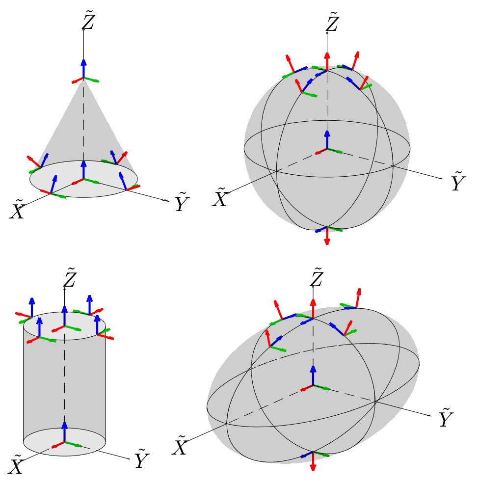
Fig. 2.14 Coordinate system behavior near the \(\tilde{Z}\) axis. \(\hat{r}\) is red, \(\hat{s}\) is green, and \(\hat{t}\) is blue.

2.1.10. Moving Coordinate System Syntax

BEGIN RECTANGULAR COORDINATE SYSTEM <string>csname
  ORIGIN CENTROID  = <ENTITY_NAME> # Name of block, surface, or nodeset
  CENTROID CALCULATION = MASS_WEIGHTED|UNWEIGHTED (MASS_WEIGHTED)
  SYSTEM = MOVING
  INITIAL CONFIGURATION = BLOCK_ALIGNED|GLOBAL_XYZ (GLOBAL_XYZ)
  OUTPUT VECTOR FIELDS = ON
END

BEGIN RECTANGULAR COORDINATE SYSTEM <string>csname
  ORIGIN = <real> <real> <real>
  Z POINT = <real> <real> <real>  # Point on Z-tilde axis
  XZ POINT = <real> <real> <real> # Point on X-tilde-Z-tilde plane
  SYSTEM = MOVING
  TRACKING ENTITY  = <ENTITY_NAME> # Name of block, surface, or nodeset
  OUTPUT VECTOR FIELDS = ON
END

BEGIN RECTANGULAR COORDINATE SYSTEM <string>csname
  ORIGIN NODESET  = <nodelist>    # Single-node nodesets
  Z POINT NODESET  = <nodelist>   # Node on Z-tilde axis
  XZ POINT NODESET = <nodelist>   # Node on X-tilde-Z-tilde plane
  SYSTEM = MOVING
  TRACKING ENTITY  = <ENTITY_NAME> # Name of block, surface, or nodeset
  OUTPUT VECTOR FIELDS = ON
END

Sierra/SM also allows the user to define a moving coordinate system using the above syntax.

If the syntax in the first code block is used, the origin of the coordinate system will be computed as the centroid of all of the nodal positions of the entity specified via the ORIGIN CENTROID line command. The entity may either be a mesh block, surface, or nodeset. The CENTROID CALCULATION can either be computed as a MASS_WEIGHTED centroid or an UNWEIGHTED centroid. The coordinate system is specified as a moving coordinate system via the SYSTEM = MOVING line command. The initial configuration of the directions of the coordinate system can be specified via the INITIAL CONFIGURATION line command. If the GLOBAL_XYZ option is used, the vectors will align with the global coordinate system directions. If the BLOCK_ALIGNED option is used, the vectors will align with the dimensions of the defined entity (block, surface, or nodeset). The r direction will align with the longest dimension of the entity, the t direction will align with the second longest dimension, and the s direction will be computed as the cross product between the two vectors.

If the syntax in the second code block is used, the origin of the coordinate system is specified via the ORIGIN line command. The other two directions are computed via the Z POINT and XZ POINT line commands. If the syntax in the third code block is used, the origin of the coordinate system is specified via the ORIGIN NODESET line command. The other two directions are computed via the Z POINT NODESET and XZ POINT NODESET line commands. In either case, the coordinate system is specified as a moving coordinate system via the SYSTEM = MOVING line command. The TRACKING ENTITY line command is used to specify which mesh entity (block, surface, or nodeset) the coordinate system will move with. When nodesets are used to specify the position and orientation of the coordinate system, the specified nodeset must contain a single node. The relevant locations are determined by the location of this single node and will be determined after potential mesh modifications using the INITIAL MESH MODIFICATION capability. Note that it is a parse error to mix explicitly defined points with nodeset-based points, i.e. Z POINT NODESET may not be used in combination with ORIGIN, for example.

The computed coordinate system directions may be visualized in the results file if the OUTPUT VECTOR FIELDS = ON command is specified. If this is specified, three nodal variables will be created for each coordinate system labeled as csname_rdir, csname_sdir, and csname_tdir. Note that these fields are only defined and updated on the tracking entities, and are zero everywhere else.

If all elements on the block, surface, or nodeset specified by the TRACKING ENTITY or ORIGIN CENTROID commands are killed via element death, each component of coordinate system will be zeroed-out since its values are no longer valid. The direction fields can be visualized by the command OUTPUT VECTOR FIELDS = ON.

2.1.11. Define Coordinate System Line Command

DEFINE COORDINATE SYSTEM <string>coord_sys_name
  <string>coord_sys_type WITH POINT <string>point_1
  POINT <string>point_2 POINT <string>point_3

The line command DEFINE COORDINATE SYSTEM can also be used to define the axis directions of a local coordinate system to be located at nodes, element centroids, or element integration points. In this command

• The string coord_sys_name is a name for this coordinate system. This name must be unique to all other coordinate systems defined in the input file.

• The string coord_sys_type states the type of the coordinate system to be used. Three options are allowed for constructing a local coordinate system: RECTANGULAR, CYLINDRICAL, and SPHERICAL.

• The strings point_1, point_2, and point_3 are the names for three points defined in the input file via DEFINE POINT command lines. These three points are used to define two of the coordinate system axes as described below for the different types of systems.

For a rectangular system, the local \(Z'\) axis is parallel to the vector from the point_1 to point_2. The local \(X'\) axis is the component of the vector from point_1 to point_3 that is orthogonal to the \(Z'\) axis. Finally, the local \(Y'\) axis is obtained from the cross product of \(Z'\) and \(X'\).

Likewise, for a cylindrical system, the local \(Z'\) axis is parallel to the vector from the point_1 to point_2 and defines the axis of the cylinder. The local \(X'\) axis is constructed as the vector normal to the cylindrical axis and passing through the location at which the local system is desired. This local point may be a node, an element centroid, or an element integration point. If this local point lies on the \(Z'\) axis, then the point point_3 is instead used to define the \(X'\) axis. Finally, the \(Y'\) axis is obtained from the cross product of \(Z'\) and \(X'\). Thus at the desired point not on the cylinder axis, the \(X'\) axis is through the cylinder thickness, \(Y'\) is tangent to the cylinder, and \(Z'\) is parallel to the cylinder axis.

For a spherical system, point_1 specifies the center of a sphere. The local \(X'\) axis is constructed as the vector from point_1 through the location at which the local system is desired. This local point may be a node, an element centroid, or an element integration point. The local \(Z'\) axis is the component of the vector from the point_1 to point_2 that is normal to the \(X'\) axis. If this \(Z'\) is parallel the \(X'\) axis, then point_3 is used instead. Finally, the \(Y'\) axis is obtained from the cross product of \(Z'\) and \(X'\). Thus at a desired point, the \(X'\) axis is through the sphere thickness and the \(Y'\) and \(Z'\) axes lie in the tangent plane.