5.2. Material Models
This section contains descriptions of the general fully supported materials available in Sierra/SM. Additional models relevant to shock problems are described in the separate Sierra/SM ITAR User’s Guide: Addendum for Shock Capabilities. Also, additional experimental, in-development, and specialty models may be found in the Sierra/SM Capabilities in Development manual.
5.2.1. Elastic Model
BEGIN PARAMETERS FOR MODEL ELASTIC
  #
  # Elastic constants
  #
  YOUNGS MODULUS = <real>
  POISSONS RATIO = <real>
  SHEAR MODULUS  = <real>
  BULK MODULUS   = <real>
  LAMBDA         = <real>
  TWO MU         = <real>
END [PARAMETERS FOR MODEL ELASTIC]
The elastic model is a hypoelastic extension of isotropic, small-strain, linear elasticity [[1], [2], [3]]. The stress-strain response for an isotropic, elastic material is
where the Lamé constants, \(\lambda\) and \(\mu\), are given by
This model is extended to a finite-deformation, hypoelastic model by first making it a rate equation. Then the stress rate is replaced with an objective stress rate and the strain rate is replaced with the rate of deformation. This gives us
The stress rate is arbitrary, as long as it is objective. Two objective stress rates are commonly used: the Jaumann rate and the Green-McInnis rate. For problems with fixed principal axes of deformation, these two rates give the same answers. For problems where the principal axes of deformation rotate during the deformation, the two rates can give different answers. Generally speaking there is no reason to pick one objective rate over another. Sierra/SM uses the Green-McInnis rate.
The fourth-order elastic moduli are used in many constitutive models. There are many equivalent representations for the elastic moduli. In index notation we present the following three representations
where \(K\) is the elastic bulk modulus and is given by
See Section 5.1.5 for more information on elastic constants input.
There are no output variables available for the elastic model. For information about the elastic model, consult [[4]].
5.2.2. Thermoelastic Model
BEGIN PARAMETERS FOR MODEL THERMOELASTIC
  #
  # Elastic constants
  #
  YOUNGS MODULUS = <real>
  POISSONS RATIO = <real>
  SHEAR MODULUS  = <real>
  BULK MODULUS   = <real>
  LAMBDA         = <real>
  TWO MU         = <real>
  #
  # Thermoelastic functions
  #
  YOUNGS MODULUS FUNCTION = <string> ym_function_name
  POISSONS RATIO FUNCTION = <string> pr_function_name
END [PARAMETERS FOR MODEL THERMOELASTIC]
The thermoelastic material model is used to describe a temperature-dependent linear elastic material. This is a hypoelastic model generally valid for small strains.
In the above command blocks:
See Section 5.1.5 for more information on elastic constants input.
The
YOUNGS MODULUS FUNCTIONcommand line references the name of a function defined in aFUNCTIONcommand line in the SIERRA scope. The function defines a scale factor on Young’s modulus as a function of temperature.The
POISSONS RATIO FUNCTIONcommand line references the name of a function defined in aFUNCTIONcommand line in the SIERRA scope. The function defines a scale factor on Poisson’s ratio as a function of temperature.
For information about the thermoelastic model, consult [[4]]. Several plasticity models share the same underlying implementation. Output state variables available for this model are listed in Table 5.9. Note, depending on options used (temperature dependence of properties, failure, etc.) some of these state variables may not be computed.
5.2.3. Neo-Hookean Model
BEGIN PARAMETERS FOR MODEL NEO_HOOKEAN
  #
  # Elastic constants
  #
  YOUNGS MODULUS = <real>
  POISSONS RATIO = <real>
  SHEAR MODULUS  = <real>
  BULK MODULUS   = <real>
  LAMBDA         = <real>
  TWO MU         = <real>
END [PARAMETERS FOR MODEL NEO_HOOKEAN]
The neo-Hookean model is a hyperelastic generalization of isotropic, small-strain linear elasticity. The stress-strain response for the neo-Hookean model may be determined from a free energy function - in this case the strain energy density, \(W\). The form of the strain energy density ([[5]]) is
where \(K\) and \(\mu\) are the bulk and shear moduli, respectively. The deformation measure is given by \(C_{ij}\), the components of the right Cauchy-Green tensor, where \(C_{ij} = F_{ki}F_{kj}\). The determinant of the deformation gradient is given by \(J\) and is a measure of the volumetric part of the deformation. \(\bar{C}_{ij}\) provides the isochoric part of the deformation and is given by
The second Piola-Kirchoff stress, with components \(S_{ij}\), may be determined by taking a derivative of the strain energy density and the Cauchy stress may be found by mapping from the second Piola-Kirchoff stress. The components of the Cauchy stress are
where \(B_{ij} = F_{ik}F_{jk}\), are the components of the left Cauchy-Green tensor and \(\delta_{ij}\) is the Kronecker delta.
Linearizing (5.3) we recover small strain linear elasticity
The neo-Hookean model is used for the recoverable (elastic) part for a number of inelastic, finite deformation constitutive models.
There are no output variables available for the neo-Hookean model.
5.2.4. Elastic Fracture Model
BEGIN PARAMETERS FOR MODEL ELASTIC_FRACTURE
  #
  # Elastic constants
  #
  YOUNGS MODULUS = <real>
  POISSONS RATIO = <real>
  SHEAR MODULUS  = <real>
  BULK MODULUS   = <real>
  LAMBDA         = <real>
  TWO MU         = <real>
  #
  # Fracture parameters
  #
  MAX STRESS                    = <real>
  CRITICAL CRACK OPENING STRAIN = <real>
END [PARAMETERS FOR MODEL ELASTIC_FRACTURE]
The elastic fracture model is linear elastic model with a simple failure model using a maximum-principal-stress failure criterion. Post failure, the stress decays isotropically based on additional strain parallel to the maximum principal stress. The critical crack opening strain, \(\varepsilon_{ccos}\) is the value of the component of strain over which the stress is decayed to zero. This strain parameter can be adjusted so that failure is mesh independent.
In the above command blocks:
See Section 5.1.5 for more information on elastic constants input.
The maximum principal stress at which failure occurs is defined with the
MAX STRESScommand line.The component of strain over which the stress decays to zero is defined with the
CRITICAL CRACK OPENING STRAINcommand line. This component of strain is aligned with the maximum-principal-stress direction at failure.
Output variables available for this model are listed in Table Table 5.1.
Name |
Variable Description |
|---|---|
|
Critical value of opening strain |
|
Crack opening direction - vector |
|
Crack opening direction - x component |
|
Crack opening direction - y component |
|
Crack opening direction - z component |
|
Value of maximum principal stress |
|
Von Mises stress at failure |
|
Stress tensor pressure at failure |
|
Maximum principal stress (UQ) |
|
Critical crack opening strain (UQ) |
5.2.5. Elastic-Plastic Model
BEGIN PARAMETERS FOR MODEL ELASTIC_PLASTIC
  #
  # Elastic constants
  #
  YOUNGS MODULUS = <real>
  POISSONS RATIO = <real>
  SHEAR MODULUS  = <real>
  BULK MODULUS   = <real>
  LAMBDA         = <real>
  TWO MU         = <real>
  #
  # Hardening Behavior
  #
  YIELD STRESS      = <real>
  BETA              = <real> (1.0)
  HARDENING MODULUS = <real>
END [PARAMETERS FOR MODEL ELASTIC_PLASTIC]
The elastic-plastic model is a hypoelastic, rate-independent linear hardening plasticity model. The rate form of the constitutive equation assumes an additive split of the rate of deformation into an elastic and plastic part
The stress rate only depends on the elastic strain rate in the problem
where \(\mathbb{C}_{ijkl}\) are the components of the fourth-order, isotropic elasticity tensor.
The key to the model is finding the plastic rate of deformation. For associated flow the plastic rate of deformation is in a direction normal to the yield surface. The yield surface is given by
where \(\phi\) is the effective stress, \(\alpha_{ij}\) are the components of the back stress (used with kinematic hardening), and \(\bar{\sigma}\) is the hardening function which is a function of an internal state variable, the equivalent plastic strain \(\bar{\varepsilon}^{p}\). An example of such a yield surface (plotted in the deviatoric \(\pi\)-plane) is presented below in Fig. 5.4. The isotropy of the yield surface is clearly evident.
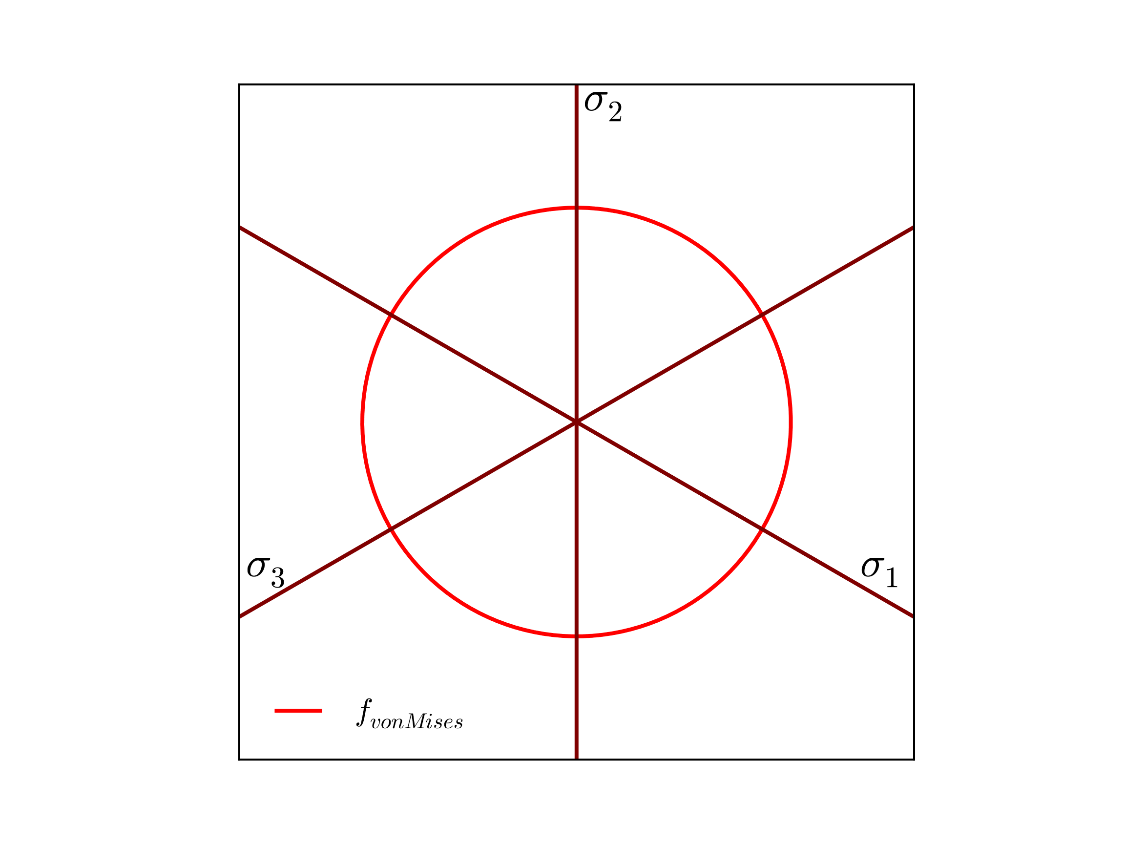
Fig. 5.4 Example von Mises yield surface (\(J_2\)) used by the elastic-plastic model presented in the deviatoric \(\pi\)-plane. In this case the surface is plotted for \(\alpha_{ij}=0\) and \(\bar{\varepsilon}^p=0\).
For the elastic plastic model a linear hardening law is assumed
where \(\sigma_{y}\) is the yield stress and \(H^{\prime}\) is the hardening modulus. If the stress state is such that \(f < 0\), the the behavior of the material is elastic; if the stress state is such that \(f = 0\) and \(\dot{f} < 0\), i.e. the strain rate brings the stress inside the yield surface, then the behavior of the material is elastic; if the stress state is such that \(f = 0\) and \(\dot{f} > 0\), i.e. the strain rate brings the stress outside the yield surface, then plastic deformation occurs.
We assume associated flow in this model, which gives the plastic rate of deformation
where \(\dot{\gamma}\) is the consistency parameter. For the elastic-plastic model the yield surface is assumed to be a von Mises yield surface with a back stress tensor to denote the center of the yield surface. The effective stress for a von Mises yield surface is
where \(s_{ij}\) are the components of the deviatoric stress tensor
and \(\alpha_{ij}\) are the components of the back stress tensor, another internal state variable.
The equivalent plastic strain is found through equating the rate of plastic work
Finally, the model allows for kinematic hardening through the back stress. The back stress is a symmetric, deviatoric rank two tensor that evolves in the following manner
The radius of the yield surface can be defined, \(R = \sqrt{\xi_{ij}\xi_{ij}}\). The evolution of the radius of the yield surface is given by
In (5.13) and (5.14) the parameter \(\beta \in [0,1]\) distributes the hardening between isotropic and kinematic hardening. If \(\beta = 1\) the hardening is isotropic, if \(\beta = 0\) the hardening is kinematic, and if \(\beta\) is between 0 and 1 the hardening is a combination of isotropic and kinematic. In the above command blocks:
See Section 5.1.5 for more information on elastic constants input. The elastic constants describe both the pre-yield behavior of the model and the slope of post yield unloading.
The yield stress, the stress at which yield first initiates, is defined with the
YIELD STRESScommand line.The hardening modulus, the slope of the post yield hardening curve, is defined with the
HARDENING MODULUScommand line.The beta parameter defines if hardening is isotropic or kinematic. See Section 5.1.6 for details on the beta parameter.
Output variables available for this model are listed in Table 5.2 and Table 5.3. For information about the elastic-plastic model, consult [[4]].
Name |
Description |
|---|---|
|
equivalent plastic strain, \(\bar{\varepsilon}^{p}\) |
|
radius of the yield surface, \(R\) |
|
back stress (symmetric tensor), \(\alpha_{ij}\) |
Name |
Description |
|---|---|
|
equivalent plastic strain, \(\bar{\varepsilon}^{p}\) |
|
equivalent plastic strain only accumulated when the material is in tension (trace of stress tensor is positive) |
|
radius of the yield surface, \(R\) |
|
back stress (symmetric tensor), \(\alpha_{ij}\) |
|
radial return iterations |
|
error in plane stress iterations |
|
plane stress iterations |
|
integrated thickness strain |
5.2.6. Elastic-Plastic Power-Law Hardening Model
BEGIN PARAMETERS FOR MODEL EP_POWER_HARD
  #
  # Elastic constants
  #
  YOUNGS MODULUS = <real>
  POISSONS RATIO = <real>
  SHEAR MODULUS  = <real>
  BULK MODULUS   = <real>
  LAMBDA         = <real>
  TWO MU         = <real>
  #
  # Hardening behavior
  #
  YIELD STRESS       = <real>
  HARDENING CONSTANT = <real>
  HARDENING EXPONENT = <real>
  LUDERS STRAIN      = <real>
END [PARAMETERS FOR MODEL EP_POWER_HARD]
The elastic-plastic power law hardening model is a hypoelastic, rate-independent plasticity model with power law hardening [[6]]. The rate form of the constitutive equation assumes an additive split of the rate of deformation into an elastic and plastic part
The stress rate only depends on the elastic strain rate in the problem
where \(\mathbb{C}_{ijkl}\) are the components of the fourth-order, isotropic elasticity tensor.
The key to integrating the model is finding the plastic rate of deformation. For associated flow the plastic rate of deformation is in a direction normal to the yield surface. The yield surface is given by
where \(\phi\) is the equivalent stress and \(\bar{\sigma}\) is the hardening function which is a function of the equivalent plastic strain \(\bar{\varepsilon}^{p}\). For this model the hardening function uses a power law
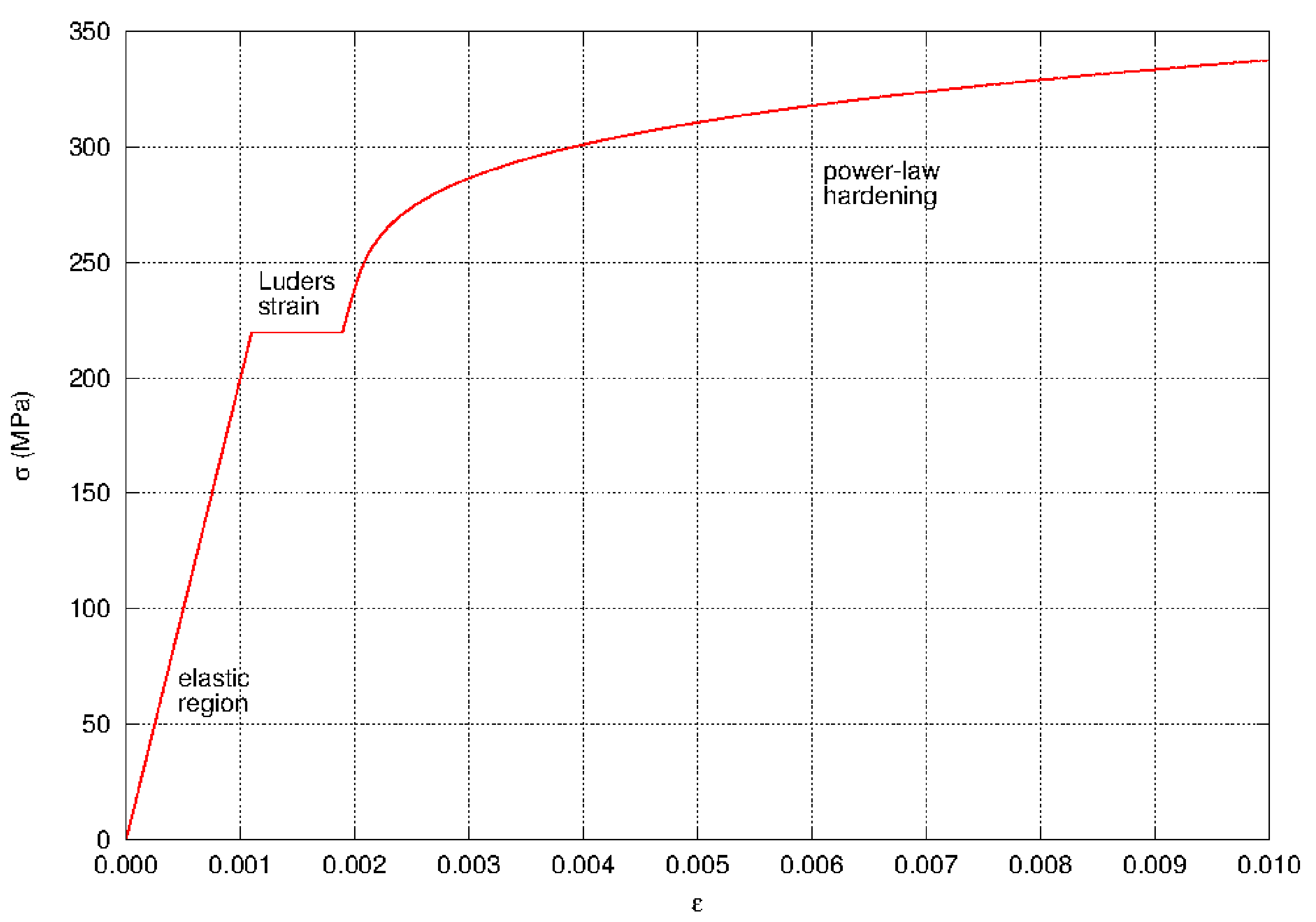
Fig. 5.5 Typical stress-strain response for the power-law hardening model.
which is shown in Fig. 5.5. The yield stress is \(\sigma_{y}\), the hardening constant is \(A\), the hardening exponent is \(n\), and the L"{u}ders strain is \(\varepsilon_{L}\). The bracket \(<\cdot>\) is the Macaulay bracket defined as
By assuming associated plastic flow, the plastic rate of deformation can be written as
For this model the yield surface is chosen to be a von Mises yield surface, so
where \(s_{ij}\) are the components of the deviatoric stress
Unlike the elastic-plastic model Section 5.2.5, the power-law hardening model does not allow for kinematic hardening, so there is no back stress.
In the above command blocks:
See Section 5.1.5 for more information on elastic constants input.
The
YIELD STRESSis the stress at which the plastic power law yielding and hardening model takes effect. See Fig. 5.5.The
LUDERS STRAINdefines a regime of zero hardening modulus prior to onset of the power law hardening. A small Luder band is seen in the hardening behavior or many metals. See Fig. 5.5 for details.The
HARDENING CONSTANTcommand line andHARDENING EXPONENTcommand define the power law hardening curve. Past the Luder strain the hardened yield surface radius is given by theHARDENING CONSTANTtimes plastic strain to theHARDENING EXPONENTpower.
Output variables available for this model are listed in Table 5.4 and Table 5.5. For information about the elastic-plastic power-law hardening model, consult [[4]].
Name |
Description |
|---|---|
|
equivalent plastic strain, \(\bar{\varepsilon}^{p}\) |
|
equivalent plastic strain only accumulated when the material is in tension (trace of stress tensor is positive) |
|
radius of yield surface, \(R\) |
|
number of radial return iterations |
Name |
Description |
|---|---|
|
equivalent plastic strain, \(\bar{\varepsilon}^{p}\) |
|
equivalent plastic strain only accumulated when the material is in tension (trace of stress tensor is positive) |
|
radius of yield surface, \(R\) |
|
number of radial return iterations |
|
error in plane stress iterations |
|
plane stress iterations |
5.2.7. Ductile Fracture Model
BEGIN PARAMETERS FOR MODEL DUCTILE_FRACTURE
  #
  # Elastic constants
  #
  YOUNGS MODULUS = <real>
  POISSONS RATIO = <real>
  SHEAR MODULUS  = <real>
  BULK MODULUS   = <real>
  LAMBDA         = <real>
  TWO MU         = <real>
  #
  # Yield surface parameters
  #
  YIELD STRESS       = <real>
  HARDENING CONSTANT = <real>
  HARDENING EXPONENT = <real>
  LUDERS STRAIN      = <real>
  #
  # Failure parameters
  #
  CRITICAL TEARING PARAMETER    = <real>
  CRITICAL CRACK OPENING STRAIN = <real>
END [PARAMETERS FOR MODEL DUCTILE_FRACTURE]
The ductile fracture model is identical to the elastic-plastic power-law hardening model with the addition of a failure criterion and an isotropic decay of the stress to zero during the failure process within the constitutive model. To accomplish this task, the tearing parameter, \(t_p\), proposed by Wellman [[7]] is introduced and the functional form as given as
where \(\sigma_{\max }\) is the maximum principal stress, and \(\sigma _{m}\) is the mean stress. It can also be noted that the tearing parameter evolves during the plastic deformation regime as indicated by integrating over the effective plastic strain, \(\bar{\varepsilon}^{p}\). The angle brackets denoting the Macaulay brackets, where
are used to ensure that the failure process occurs only with tensile stress states and prevent “damage healing”. The failure process then initiates at a critical tearing parameter, \(t_p^{\text{crit}}\), and the corresponding stress decay occurs over a strain interval corresponding to the critical crack opening strain, \(\varepsilon_{\text{ccos}}\). Importantly, the \(\varepsilon_{\text{ccos}}\) serves a dual role in that it may also be used to control the energy dissipated during failure. With respect to the latter point, careful selection of the critical crack opening strain may be used to ensure consistent energy is dissipated through different meshes. This decay process is isotropic and linear with the current damage value being equivalent to the ratio of crack opening strain in the direction of the maximum principal stress to the critical value.
In the above command blocks:
See Section 5.1.5 for more information on elastic constants input.
The
YIELD STRESSis the stress at which the plastic power load yielding and hardening model takes effect. See Fig. 5.5.The
LUDERS STRAINdefines a regime of zero hardening modulus prior to onset of the power law hardening. A small Luder band is seen in the hardening behavior or many metals. See Fig. 5.5 for details.The
HARDENING CONSTANTcommand line andHARDENING EXPONENTcommand define the power law hardening curve. Past the Luder strain the hardened yield surface radius is given by theHARDENING CONSTANTtimes plastic strain to theHARDENING EXPONENTpower.CRITICAL TEARING PARAMETERdefines the \(t_{p}\) value at which fracture and subsequent decay of stress will occur.When the model undergoes additionally strain after reaching the critical tearing parameter the stress in the model will decay to zero. The amount strain over which the stress decays to zero is defined with the
CRITICAL CRACK OPENING STRAINcommand line. The relevant opening strain is the component of strain that is aligned with the maximum-principal-stress direction at initial failure.
Output variables available for this model are listed in Table 5.6. For information about the ductile fracture material model, consult [[7]].
Name |
Description |
|---|---|
|
equivalent plastic strain, \(\bar{\varepsilon}^{p}\) |
|
radius of yield surface, \(R\) |
|
back stress - tensor \(\alpha_{ij}\) |
|
Current value of the integrated tearing parameter |
|
Current value of the crack opening strain. Will be zero prior to reaching the maximum tearing parameter. |
|
Crack opening direction (maximum principal stress direction at failure) - vector |
|
XX component of current strain |
|
YY component of current strain |
|
ZZ component of current strain |
|
XY component of current strain |
|
YZ component of current strain |
|
ZX component of current strain |
|
Yield surface radius at failure |
|
Stress pressure norm at failure |
5.2.8. Multilinear Elastic-Plastic Hardening Model
BEGIN PARAMETERS FOR MODEL MULTILINEAR_EP
  #
  # Elastic constants
  #
  YOUNGS MODULUS = <real>
  POISSONS RATIO = <real>
  SHEAR MODULUS  = <real>
  BULK MODULUS   = <real>
  LAMBDA         = <real>
  TWO MU         = <real>
  #
  # Hardening behavior
  #
  YIELD STRESS       = <real>
  BETA               = <real> (1.0)
  HARDENING FUNCTION = <string> hardening_function_name
  #
  # Functions
  #
  YOUNGS MODULUS FUNCTION = <string> ym_function_name
  POISSONS RATIO FUNCTION = <string> pr_function_name
  YIELD STRESS FUNCTION   = <string> yield_stress_function_name
END [PARAMETERS FOR MODEL MULTILINEAR_EP]
The multilinear elastic-plastic model is a generalization of the standard rate independent plasticity models already presented - the linear and power law hardening models. However, rather than having a specific functional form, the multilinear hardening model allows the user to input a piecewise linear function for the hardening curve. The rate form of the constitutive equation assumes an additive split of the rate of deformation into an elastic and plastic part such that
The stress rate only depends on the elastic strain rate so that,
where \(\mathbb{C}_{ijkl}\) are the components of the fourth-order, isotropic elasticity tensor.
The key to the model is finding the plastic rate of deformation. For associated flow, the plastic rate of deformation is in the direction normal to the yield surface. With a yield surface given by
then the plastic rate of deformation can be written as
For this model the yield surface is taken to be a von Mises yield surface, such that
where \(s_{ij}\) are the components of the deviatoric stress
For simplicity it is easier to write (5.18) in terms of the normal to the yield surface
The model also incorporates temperature dependence in that the elastic properties and the yield stress can be functions of temperature. This is not as general as having the yield curves depend on temperature. For that behavior the thermoelastic-plastic model can be used.
An example stress vs. plastic strain hardening curve is shown in Fig. 5.6. This curve was generated for a loading case of uniaxial strain. In this case, the effective stress is the same as the uniaxial. Therefore, for use with the multilinear elastic-plastic model this curve would simply have to be discretized and used as input.
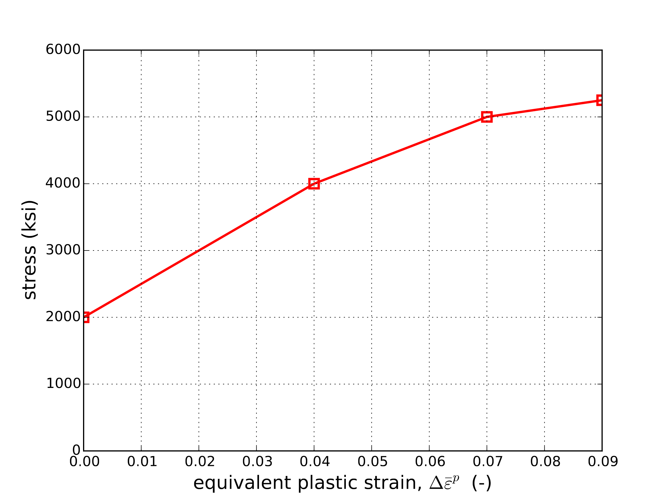
Fig. 5.6 An example of a multilinear elastic-plastic stress-strain curve.
In the above command blocks:
See Section 5.1.5 for more information on elastic constants input.
The beta parameter defines if hardening is isotropic or kinematic. See Section 5.1.6 for details on the beta parameter.
YIELD STRESSdefines the stress where plastic yielding first occurs.The
HARDENING FUNCTIONcommand line references the name of a function defined in aFUNCTIONcommand line in the SIERRA scope. The function describes the hardening behavior of the material as stress versus equivalent plastic strain. The x values of the function should be values of equivalent plastic strain while the y values of the function can be either the increment of stress over the yield stress or the actual stress at the corresponding equivalent plastic strain. Note the hardening function can have its first point defined at (0,0), or at (0,YIELD_STRESS). Either function definition behaves the same as only the slope of the hardening function between two strains is used by the model.The
YOUNGS MODULUS FUNCTIONcommand line references the name of a function defined in aFUNCTIONcommand line in the SIERRA scope that describes a scale factor on Young’s modulus as a function of temperature.The
POISSONS RATIO FUNCTIONcommand line references the name of a function defined in aFUNCTIONcommand line in the SIERRA scope that describes a scale factor on Poisson’s ratio as a function of temperature.The
YIELD STRESS FUNCTIONcommand line references the name of a function defined in aFUNCTIONcommand line in the SIERRA scope that describes a scale factor on the yield stress as a function of temperature.
Output variables available for this model are listed in Table 5.7 and Table 5.8.
Name |
Description |
|---|---|
|
equivalent plastic strain |
|
equivalent plastic strain only accumulated when the material is in tension (trace of stress tensor is positive) |
|
radius of yield surface |
|
back stress (symmetric tensor) |
|
the current Young’s modulus as a function of temperature |
|
the current Poisson’s ratio as a function of temperature |
|
the current yield stress as a function of temperature |
|
radial return iterations |
|
inside (0) or on (1) the yield surface |
Name |
Description |
|---|---|
|
equivalent plastic strain |
|
equivalent plastic strain only accumulated when the material is in tension (trace of stress tensor is positive) |
|
radius of yield surface |
|
back stress (symmetric tensor) |
|
the current Young’s modulus as a function of temperature |
|
the current Poisson’s ratio as a function of temperature |
|
the current yield stress as a function of temperature |
|
radial return iterations |
|
error in plane stress iterations |
|
plane stress iterations |
5.2.9. Multilinear Elastic-Plastic Hardening Model with Failure
BEGIN PARAMETERS FOR MODEL ML_EP_FAIL
  #
  # Elastic constants
  #
  YOUNGS MODULUS = <real>
  POISSONS RATIO = <real>
  SHEAR MODULUS  = <real>
  BULK MODULUS   = <real>
  LAMBDA         = <real>
  TWO MU         = <real>
  #
  # Hardening behavior
  #
  YIELD STRESS       = <real>
  BETA               = <real> (1.0)
  HARDENING FUNCTION = <string> hardening_function_name
  #
  # Functions
  #
  YOUNGS MODULUS FUNCTION = <string> ym_function_name
  POISSONS RATIO FUNCTION = <string> pr_function_name
  YIELD STRESS FUNCTION   = <string> yield_stress_function_name
  #
  # Failure parameters
  #
  CRITICAL TEARING PARAMETER    = <real>
  CRITICAL CRACK OPENING STRAIN = <real>
  CRITICAL BIAXIALITY RATIO     = <real> critical_ratio(0.0)
  FAILURE EXPONENT              = <real> (4.0)
END [PARAMETERS FOR MODEL ML_EP_FAIL]
Like the ductile fracture model, the multilinear elastic-plastic fail model is an extension of an existing plasticity model (multilinear elastic-plastic) to include a ductile failure criteria. Again, the tearing parameter criterion and failure propagation model of Wellman [[7]] is selected. Specifically, this approach uses a failure criterion (the tearing parameter, \(t_p\)) that is based on the history of the plastic strain and stress states. Most failure criteria for ductile failure involve some form of the stress triaxiality, or the ratio of the pressure and the effective (shear) stress. The tearing parameter, however, is slightly different in that it depends on the pressure and the maximum principal stress and is given as,
with \(\sigma_{\text{max}}\) and \(\sigma_{m}\) being the maximum principal and mean stresses, respectively. The exponent \(m\) is typically taken to be 4 while the \(\langle \cdot \rangle\) are Macaulay brackets defined as,
and introduced so that failure only occurs and propagates under tensile stress states. Failure then initiates when the tearing parameter, \(t_p\), reaches a critical value, \(t_p^{\text{crit}}\). After this point, the stress decays (to 0) in a linear fashion according to the ratio of the crack opening strain in the maximum principal stress direction to its critical value, \(\varepsilon_{\text{ccos}}\). Modification and control of this latter parameter is important as it may be used to ensure consistent energy is dissipated through different meshes.
In the above command blocks:
See Section 5.1.5 for more information on elastic constants input.
The beta parameter defines if hardening is isotropic or kinematic. See Section 5.1.6 for details on the beta parameter.
YIELD STRESSdefines the stress for onset of yielding and plasticity.The
HARDENING FUNCTIONcommand line references the name of a function defined in aFUNCTIONcommand line in the SIERRA scope. The function describes the hardening behavior of the material as stress versus equivalent plastic strain. The x values of the function should be values of equivalent plastic strain while the y values of the function can be either the increment of stress over the yield stress or the actual stress at the corresponding equivalent plastic strain. Note the hardening function can have its first point defined at (0,0), or at (0,YIELD_STRESS). Either function definition behaves the same as only the slope of the hardening function between two strains is used by the model.The
YOUNGS MODULUS FUNCTIONcommand line references the name of a function defined in aFUNCTIONcommand line in the SIERRA scope that describes a scale factor on Young’s modulus as a function of temperature.The
POISSONS RATIO FUNCTIONcommand line references the name of a function defined in aFUNCTIONcommand line in the SIERRA scope that describes a scale factor on Poisson’s ratio as a function of temperature.The
YIELD STRESS FUNCTIONcommand line references the name of a function defined in aFUNCTIONcommand line in the SIERRA scope that describes a scale factor on the yield stress as a function of temperature.CRITICAL TEARING PARAMETERdefines the \(t_{p}\) value at which fracture and subsequent decay of stress will occur.When the model undergoes additionally strain after reaching the critical tearing parameter the stress in the model will decay to zero. The amount strain over which the stress decays to zero is defined with the
CRITICAL CRACK OPENING STRAINcommand line. The relevant opening strain is the component of strain that is aligned with the maximum-principal-stress direction at initial failure.The
CRITICAL BIAXIALITY RATIOcommand line should only be used under highly specific conditions and with extreme caution. It is intended only for the special case where the stress state is nearly biaxial, resulting in nearly identical principal strains. In this case, the eigenvector computation can give unreliable results for the direction vectors for the principal strains. If the ratio of the difference between two principal strains divided by their magnitude is less that the value specified by theCRITICAL BIAXIALITY RATIOcommand, the direction of the vector defining the crack opening strain will be given equal weight in each of the principal directions associated with those strains. The default value for the critical ratio is 0.0, which means that the principal directions will be accepted directly from the eigenvector computation. This command should only be used as a last resort if the loading is nearly biaxial and the default value has been demonstrated to lead to elements with high strains that are not failing long after reaching the critical tearing parameter.The
FAILURE EXPONENTcommand line specifies the exponent on the tearing parameter, the \(m\) parameter in (5.19). This exponent defaults to 4.0.
Output variables available for this model are listed in Table 5.9 and Table 5.10.
Name |
Variable Description |
|---|---|
|
Equivalent plastic strain |
|
Radius of yield surface |
|
back stress - tensor |
|
back stress - xx component |
|
back stress - yy component |
|
back stress - zz component |
|
back stress - xy component |
|
back stress - yz component |
|
back stress - zx component |
|
Current Young’s modulus as a function of temperature |
|
Current Poisson’s ratio as a function of temperature |
|
Current Yield stress as a function of temperature |
|
equivalent plastic strain only accumulated when the material is in tension (trace of stress tensor is positive |
|
radial return iteration |
|
inside(0) or on(1) yield surface |
|
Current integrated value of the tearing parameter. Zero until yield is reached |
|
Current value of the crack opening strain. Zero until the critical tearing parameter is reached |
|
crack opening direction at failure - vector |
|
crack opening direction at failure - x component |
|
crack opening direction at failure - y component |
|
crack opening direction at failure - z component |
|
maximum radius at initial failure |
|
maximum stress pressure norm at initial failure |
|
|
|
Name |
Variable Description |
|---|---|
|
equivalent plastic strain |
|
radius of yield surface |
|
back stress - tensor |
|
back stress - xx component |
|
back stress - yy component |
|
back stress - zz component |
|
back stress - xy component |
|
back stress - yz component |
|
back stress - zx component |
|
Current Young’s modulus as a function of temperature |
|
Current Poisson’s ratio as a function of temperature |
|
Current Yield stress as a function of temperature |
|
radial return iterations |
|
Error in plane stress iterations |
|
Plane stress iterations |
|
Current integrated value of the tearing parameter. Zero until yield is reached |
|
Current value of the crack opening strain. Zero until the critical tearing parameter is reached |
|
crack opening direction at failure - vector |
|
crack opening direction at failure - x component |
|
crack opening direction at failure - y component |
|
crack opening direction at failure - z component |
|
maximum radius at initial failure |
|
equivalent plastic strain only accumulated when the material is in tension (trace of stress tensor is positive) |
5.2.10. Elastic-Plastic Hardening Model with Failure
BEGIN PARAMETERS FOR MODEL ELASTIC_PLASTIC_FAIL
  #
  # Elastic constants
  #
  YOUNGS MODULUS = <real>
  POISSONS RATIO = <real>
  SHEAR MODULUS  = <real>
  BULK MODULUS   = <real>
  LAMBDA         = <real>
  TWO MU         = <real>
  #
  # Isotropic/Kinematic hardening factor
  #
  BETA         = <real> (1.0)
  YIELD STRESS = <real>
  HARDENING FUNCTION      = <string>hardening_function_name
  POISSONS RATIO FUNCTION = <string>pr_function_name
  YIELD STRESS FUNCTION   = <string>yield_stress_function_name
  YOUNGS MODULUS FUNCTION = <string>ym_function_name
  #
  # Failure parameters
  #
  CRITICAL TEARING PARAMETER    = <real>crit_tearing
  CRITICAL CRACK OPENING STRAIN = <real>critical_strain
END [PARAMETERS FOR MODEL ELASTIC_PLASTIC_FAIL]
This model behaves identical to the ML_EP_FAIL (Section 5.2.9) material mode and only exists for legacy syntax compatibility purposes.
5.2.11. Thermoelastic-Plastic Model
BEGIN PARAMETERS FOR MODEL THERMOELASTIC_PLASTIC
  #
  # Elastic constants
  #
  YOUNGS MODULUS = <real>
  POISSONS RATIO = <real>
  SHEAR MODULUS  = <real>
  BULK MODULUS   = <real>
  LAMBDA         = <real>
  TWO MU         = <real>
  #
  # Isotropic/Kinematic hardening factor
  #
  BETA = <real>beta_parameter(1.0)
  YIELD STRESS = <real>yield_stress
  YOUNGS MODULUS FUNCTION = <string>ym_function_name
  POISSONS RATIO FUNCTION = <string>pr_function_name
  YIELD STRESS FUNCTION = <string>ys_function_name
  TEMPERATURES = <real(s)>temperature_values
  HARDENING FUNCTIONS = <string(s)>hardening_functions
END [PARAMETERS FOR MODEL THERMOELASTIC_PLASTIC]
The thermoelastic-plastic model is similar to the elastic-plastic model, but allows for temperature-dependent changes of the material properties. All elastic-plastic input parameters are still valid for the thermoelastic-plastic model, in addition to the temperature dependent functions.
In the above command blocks:
See Section 5.1.5 for more information on elastic constants input.
The beta parameter defines if hardening is isotropic or kinematic. See Section 5.1.6 for details on the beta parameter.
The yield stress, the stress at which yield first initiates, is defined with the
YIELD STRESScommand line.The
YIELD STRESS FUNCTIONcommand line references the name of a function defined in aFUNCTIONcommand line in the SIERRA scope that describes a scale factor on Yield Stress as a function of temperature.The
YOUNGS MODULUS FUNCTIONcommand line references the name of a function defined in aFUNCTIONcommand line in the SIERRA scope that describes a scale factor on Young’s modulus as a function of temperature.The
POISSONS RATIO FUNCTIONcommand line references the name of a function defined in aFUNCTIONcommand line in the SIERRA scope that describes a scale factor on Poisson’s ratio as a function of temperature.The
TEMPERATUREScommand line specifies the temperatures that correspond to the hardening functions defined in theHARDENING FUNCTIONScommand line. The number of temperatures input here must match the number of hardening functions input.The
HARDENING FUNCTIONScommand line references the names of the functions defined in aFUNCTIONcommand line in the SIERRA scope that describes the hardening behavior for the material as stress versus equivalent plastic strain at the temperatures defined in theTEMPERATUREScommand line. The number of hardening functions input here must match the number of temperatures input. If the material temperature exactly matches one of the input temperatures the hardening of the material will exactly follow the hardening curve associated with that temperature. If the material temperature is bracketed by two hardening curves the actual hardening curve taken will be linearly interpolated between the bracketing curves. If the material temperature is either above the highest defined temperature function or below the lowest defined temperature function the closest hardening curve will be used for the material hardening.
Several plasticity models share the same underlying implementation. Output state variables available for this model are listed in Table Table 5.9. Note, depending on options used (temperature dependence of properties, failure, etc.) some of these state variables may not be computed.
5.2.12. Thermoelastic-Plastic Model with Failure
BEGIN PARAMETERS FOR MODEL THERMOELASTIC_PLASTIC_FAIL
  #
  # Elastic constants
  #
  YOUNGS MODULUS = <real>
  POISSONS RATIO = <real>
  SHEAR MODULUS  = <real>
  BULK MODULUS   = <real>
  LAMBDA         = <real>
  TWO MU         = <real>
  #
  # Isotropic/Kinematic hardening factor
  #
  BETA = <real>beta_parameter(1.0)
  TEMPERATURES = <real(s)>temperature_values
  YIELD STRESS = <real>yield_stress
  YOUNGS MODULUS FUNCTION = <string>ym_function_name
  POISSONS RATIO FUNCTION = <string>pr_function_name
  YIELD STRESS FUNCTION = <string>ys_function_name
  HARDENING FUNCTIONS = <string(s)>hardening_functions
  CRITICAL CRACK OPENING STRAIN = <real>critical_strain
  CRITICAL TEARING PARAMETER = <real>crit_tearing
  CRITICAL CRACK OPENING STRAIN FUNCTION
     = <string>crack_open_strain_function_name
  CRITICAL TEARING PARAMETER FUNCTION
     = <string>tearing_parameter_function_name
END [PARAMETERS FOR MODEL THERMOELASTIC_PLASTIC_FAIL]
The thermoelastic-plastic model with failure is similar to the ELASTIC_PLASTIC_FAIL material model, but allows for additional temperature-dependent changes of the material.
In the above command blocks:
See Section 5.1.5 for more information on elastic constants input.
The beta parameter defines if hardening is isotropic or kinematic. See Section 5.1.6 for details on the beta parameter.
YIELD STRESSdefines the stress for onset of yielding and plasticity.The
TEMPERATUREScommand line specifies the temperatures that correspond to the hardening functions defined in theHARDENING FUNCTIONScommand line. The number of temperatures input here must match the number of hardening functions input.The
HARDENING FUNCTIONScommand line references the names of the functions defined in aFUNCTIONcommand line in the SIERRA scope that describes the hardening behavior for the material as stress versus equivalent plastic strain at the temperatures defined in theTEMPERATUREScommand line. The number of hardening functions input here must match the number of temperatures input. If the material temperature exactly matches one of the input temperatures the hardening of the material will exactly follow the hardening curve associated with that temperature. If the material temperature is bracketed by two hardening curves the actual hardening curve taken will be linearly interpolated between the bracketing curves. If the material temperature is either above the highest defined temperature function or below the lowest defined temperature function the closest hardening curve will be used for the material hardening.The
POISSONS RATIO FUNCTIONcommand line references the name of a function defined in aFUNCTIONcommand line in the SIERRA scope that describes a scale factor on Poisson’s ratio as a function of temperature.The
YIELD STRESS FUNCTIONcommand line references the name of a function defined in aFUNCTIONcommand line in the SIERRA scope that describes a scale factor on the yield stress as a function of temperature.CRITICAL TEARING PARAMETERdefines the \(t_{p}\) value at which fracture and subsequent decay of stress will occur.When the model undergoes additionally strain after reaching the critical tearing parameter the stress in the model will decay to zero. The amount strain over which the stress decays to zero is defined with the
CRITICAL CRACK OPENING STRAINcommand line. The relevant opening strain is the component of strain that is aligned with the maximum-principal-stress direction at initial failure.The
CRITICAL CRACK OPENING STRAIN FUNCTION `` command line references the name of a function defined in a ``FUNCTIONcommand line in the SIERRA scope that describes a scale factor on the crack opening strain as a function of temperature.The
CRITICAL TEARING PARAMETER FUNCTIONcommand line references the name of a function defined in aFUNCTIONcommand line in the SIERRA scope that describes a scale factor on the tearing parameter as a function of temperature.
Several plasticity models share the same underlying implementation. Output state variables available for this model are listed in Table Table 5.9. Note, depending on options used (temperature dependence of properties, failure, etc.) some of these state variables may not be computed.
5.2.13. J2 Plasticity Model
BEGIN PARAMETERS FOR MODEL J2_PLASTICITY
  #
  # Elastic constants
  #
  YOUNGS MODULUS = <real>
  POISSONS RATIO = <real>
  SHEAR MODULUS  = <real>
  BULK MODULUS   = <real>
  LAMBDA         = <real>
  TWO MU         = <real>
  #
  # Yield surface parameters
  #
  YIELD STRESS = <real>
  BETA         = <real> (1.0)
  #
  # Hardening model
  #
  HARDENING MODEL = LINEAR | POWER_LAW | VOCE | USER_DEFINED |
  FLOW_STRESS | DECOUPLED_FLOW_STRESS | JOHNSON_COOK |
  POWER_LAW_BREAKDOWN
  #
  # Linear hardening
  #
  HARDENING MODULUS = <real>
  #
  # Power-law hardening
  #
  HARDENING CONSTANT = <real>
  HARDENING EXPONENT = <real> (0.5)
  LUDERS STRAIN      = <real> (0.0)
  #
  # Voce hardening
  #
  HARDENING MODULUS       = <real>
  EXPONENTIAL COEFFICIENT = <real>
  #
  # Johnson-Cook hardening
  #
  HARDENING FUNCTION = <string>hardening_function_name
  RATE CONSTANT      = <real>
  REFERENCE RATE     = <real>
  #
  # Power law breakdown hardening
  #
  HARDENING FUNCTION = <string>hardening_function_name
  RATE COEFFICIENT   = <real>
  RATE EXPONENT      = <real>
  # User defined hardening
  #
  HARDENING FUNCTION = <string>hardening_function_name
  #
  #
  # Following Commands Pertain to Flow_Stress Hardening Model
  #
  #    -  Isotropic Hardening model
  #
  ISOTROPIC HARDENING MODEL = LINEAR | POWER_LAW | VOCE |
                              USER_DEFINED
  #
  # Specifications for Linear, Power-law, and Voce same as above
  #
  # User defined hardening
  #
  ISOTROPIC HARDENING FUNCTION = <string>iso_hardening_fun_name
  #
  #     - Rate dependence
  #
  RATE MULTIPLIER = JOHNSON_COOK | POWER_LAW_BREAKDOWN |
     USER_DEFINED | RATE_INDEPENDENT (RATE_INDEPENDENT)
  #
  # Specifications for Johnson-Cook, Power-law-breakdown
  #     same as before EXCEPT no need to specify a
  #     hardening function
  #
  # User defined rate multiplier
  #
  RATE MULTIPLIER FUNCTION = <string> rate_mult_function_name
  #
  #     - Temperature dependence
  #
  TEMPERATURE MULTIPLIER = JOHNSON_COOK | USER_DEFINED |
     TEMPERATURE_INDEPENDENT (TEMPERATURE_INDEPENDENT)
  #
  #  Johnson-Cook temperature dependence
  #
  MELTING TEMPERATURE   = <real>
  REFERENCE TEMPERATURE = <real>
  TEMPERATURE EXPONENT  = <real>
  #
  #  User-defined temperature dependence
  TEMPERATURE MULTIPLIER FUNCTION = <string>temp_mult_function_name
  #
  # Following Commands Pertain to Decoupled_Flow_Stress Hardening Model
  #
  #    -  Isotropic Hardening model
  #
  ISOTROPIC HARDENING MODEL = LINEAR | POWER_LAW | VOCE | USER_DEFINED
  #
  # Specifications for Linear, Power-law, and Voce same as above
  #
  # User defined hardening
  #
  ISOTROPIC HARDENING FUNCTION = <string>isotropic_hardening_function_name
  #
  #     - Rate dependence
  #
  YIELD RATE MULTIPLIER = JOHNSON_COOK | POWER_LAW_BREAKDOWN |
              USER_DEFINED | RATE_INDEPENDENT (RATE_INDEPENDENT)
  #
  # Specifications for Johnson-Cook, Power-law-breakdown same as before
  #     EXCEPT no need to specify a hardening function
  #     AND should be preceded by YIELD
  #
  #     As an example for Johnson-Cook yield rate dependence,
  #
  YIELD RATE CONSTANT  = <real>
  YIELD REFERENCE RATE = <real>
  #
  # User defined rate multiplier
  #
  YIELD RATE MULTIPLIER FUNCTION = <string>yield_rate_mult_function_name
  #
  HARDENING_RATE MULTIPLIER = JOHNSON_COOK | POWER_LAW_BREAKDOWN |
              USER_DEFINED | RATE_INDEPENDENT (RATE_INDEPENDENT)
  #
  #     Syntax same as for yield parameters but with a HARDENING prefix
  #
  #     - Temperature dependence
  #
  YIELD TEMPERATURE MULTIPLIER = JOHNSON_COOK | USER_DEFINED |
            TEMPERATURE_INDEPENDENT (TEMPERATURE_INDEPENDENT)
  #
  #  Johnson-Cook temperature dependence
  #
  YIELD MELTING TEMPERATURE   = <real>
  YIELD REFERENCE TEMPERATURE = <real>
  YIELD TEMPERATURE EXPONENT  = <real>
  #
  #  User-defined temperature dependence
  YIELD TEMPERATURE MULTIPLIER FUNCTION = <string>yield_temp_mult_fun_name
  #
  HARDENING TEMPERATURE MULTIPLIER = JOHNSON_COOK | USER_DEFINED |
            TEMPERATURE_INDEPENDENT (TEMPERATURE_INDEPENDENT)
  #
  #   Syntax for hardening constants same as for yield but
  #            with HARDENING prefix
  #
  # Optional Failure Definitions
  #    Following only need to be defined if intend to use failure model
  #
  FAILURE MODEL = TEARING_PARAMETER | JOHNSON_COOK_FAILURE | WILKINS
                  | MODULAR_FAILURE | MODULAR_BCJ_FAILURE

  CRITICAL FAILURE PARAMETER = <real>
  #
  # TEARING_PARAMETER Failure model definitions
  #
  TEARING PARAMETER EXPONENT = <real>
  #
  # JOHNSON_COOK_FAILURE Failure model definitions
  #
  JOHNSON COOK D1       = <real>
  JOHNSON COOK D2       = <real>
  JOHNSON COOK D3       = <real>
  JOHNSON COOK D4       = <real>
  JOHNSON COOK D5       = <real>
  #
  #Following Johnson-Cook parameters can only be defined once.  As such, only
  #  needed if not previously defined via Johnson-Cook multipliers
  #  w/ flow-stress hardening.  Does need to be defined
  #  w/ Decoupled Flow Stress
  #
  REFERENCE RATE        = <real>
  REFERENCE TEMPERATURE = <real>
  MELTING TEMPERATURE   = <real>
  #
  # WILKINS Failure model definitions
  #
  WILKINS ALPHA    = <real>
  WILKINS BETA     = <real>
  WILKINS PRESSURE = <real>
  #
  #  MODULAR_FAILURE Failure model definitions
  #
  PRESSURE MULTIPLIER         = PRESSURE_INDEPENDENT | WILKINS
                                | USER_DEFINED (PRESSURE_INDEPENDENT)
  LODE ANGLE MULTIPLIER       = LODE_ANGLE_INDEPENDENT |
                                WILKINS (LODE_ANGLE_INDEPENDENT)
  TRIAXIALITY MULTIPLIER      = TRIAXIALITY_INDEPENDENT | JOHNSON_COOK
                                | USER_DEFINED (TRIAXIALITY_INDEPENDENT)
  RATE FAIL MULTIPLIER        = RATE_INDEPENDENT | JOHNSON_COOK
                                | USER_DEFINED (RATE_INDEPENDENT)
  TEMPERATURE FAIL MULTIPLIER = TEMPERATURE_INDEPENDENT | JOHNSON_COOK
                                | USER_DEFINED (TEMPERATURE_INDEPENDENT)
  #
  # Individual multiplier definitions
  #
  PRESSURE MULTIPLIER = WILKINS
  WILKINS ALPHA       = <real>
  WILKINS PRESSURE    = <real>
  #
  PRESSURE MULTIPLIER = USER_DEFINED
  PRESSURE MULTIPLIER FUNCTION = <string> pressure_multiplier_fun_name
  #
  LODE ANGLE MULTIPLIER = WILKINS
  WILKINS BETA          = <real>
  #
  TRIAXIALITY MULTIPLIER = JOHNSON_COOK
  JOHNSON COOK D1        = <real>
  JOHNSON COOK D2        = <real>
  JOHNSON COOK D3        = <real>
  #
  TRIAXIALITY MULTIPLIER = USER_DEFINED
  TRIAXIALITY MULTIPLIER FUNCTION = <string> triaxiality_multiplier_fun_name
  #
  RATE FAIL MULTIPLIER = JOHNSON_COOK
  JOHNSON COOK D4      = <real>
  # REFERENCE RATE should only be added if not previously defined
  REFERENCE RATE       = <real>
  #
  RATE FAIL MULTIPLIER = USER_DEFINED
  RATE FAIL MULTIPLIER FUNCTION = <string> rate_fail_multiplier_fun_name
  #
  TEMPERATURE FAIL MULTIPLIER = JOHNSON_COOK
  JOHNSON COOK D5             = <real>
  # JC Temperatures should only be defined if not previously given
  REFERENCE TEMPERATURE       = <real>
  MELTING TEMPERATURE         = <real>
  #
  TEMPERATURE FAIL MULTIPLIER          = USER_DEFINED
  TEMPERATURE FAIL MULTIPLIER FUNCTION = <string> temp_multiplier_fun_name
  #
  # MODULAR_BCJ_FAILURE Failure model definitions
  #
  INITIAL DAMAGE    = <real>
  INITIAL VOID SIZE = <real>
  DAMAGE BETA       = <real> (0.5)
  GROWTH MODEL      = COCKS_ASHBY | NO_GROWTH (NO_GROWTH)
  NUCLEATION MODEL  = HORSTEMEYER_GOKHALE | CHU_NEEDLEMAN_STRAIN
                      | NO_NUCLEATION (NO_NUCLEATION)
  #
  GROWTH RATE FAIL MULTIPLIER        = JOHNSON_COOK | USER_DEFINED
                                       | RATE_INDEPENDENT
                                       (RATE_INDEPENDENT)
  GROWTH TEMPERATURE FAIL MULTIPLIER = JOHNSON_COOK | USER_DEFINED
                                       | TEMPERATURE_INDEPENDENT
                                       (TEMPERATURE_INDEPENDENT)
  #
  NUCLEATION RATE FAIL MULTIPLIER        = JOHNSON_COOK | USER_DEFINED
                                           | RATE_INDEPENDENT
                                           (RATE_INDEPENDENT)
  NUCLEATION TEMPERATURE FAIL MULTIPLIER = JOHNSON_COOK | USER_DEFINED
                                           | TEMPERATURE_INDEPENDENT
                                           (TEMPERATURE_INDEPENDENT)
  #
  # Definitions for individual growth and nucleation models
  #
  GROWTH MODEL = COCKS_ASHBY
  DAMAGE EXPONENT = <real> (0.5)
  #
  NUCLEATION MODEL      = HORSTEMEYER_GOKHALE
  NUCLEATION PARAMETER1 = <real> (0.0)
  NUCLEATION PARAMETER2 = <real> (0.0)
  NUCLEATION PARAMETER3 = <real> (0.0)
  #
  NUCLEATION MODEL          = CHU_NEEDLEMAN_STRAIN
  NUCLEATION AMPLITUDE      = <real>
  MEAN NUCLEATION STRAIN    = <real>
  NUCLEATION STRAIN STD DEV = <real>
  #
  # Definitions for rate and temperature fail multiplier
  #   Note: only showing definitions for growth.
  #    Nucleation terms are the same just with NUCLEATION instead
  #    of GROWTH
  #
  GROWTH RATE FAIL MULTIPLIER = JOHNSON_COOK
  GROWTH JOHNSON COOK D4      = <real>
  GROWTH REFERENCE RATE       = <real>
  #
  GROWTH RATE FAIL MULTIPLIER          = USER_DEFINED
  GROWTH RATE FAIL MULTIPLIER FUNCTION = <string> growth_rate_fail_mult_func
  #
  GROWTH TEMPERATURE FAIL MULTIPLIER = JOHNSON_COOK
  GROWTH JOHNSON COOK D5             = <real>
  GROWTH REFERENCE TEMPERATURE       = <real>
  GROWTH MELTING TEMPERATURE         = <real>
  #
  GROWTH TEMPERATURE FAIL MULTIPLIER          = USER_DEFINED
  GROWTH TEMPERATURE FAIL MULTIPLIER FUNCTION = <string> temp_fail_mult_func
  #
  #
  # Optional Adiabatic Heating/Thermal Softening  Definitions
  #    Following only need to be defined if intend to use failure model
  #
  THERMAL SOFTENING MODEL = ADIABATIC | COUPLED
  #
  SPECIFIC HEAT = <real> # not needed for COUPLED
  BETA_TQ       = <real>
END [PARAMETERS FOR MODEL J2_PLASTICITY]
The \(J_2\) plasticity model is a generic implementation of a von Mises yield surface with kinematic and isotropic hardening features. Unlike other models (e.g. Elastic-Plastic, Elastic-Plastic Power Law) more flexible, general hardening forms are implemented enabling different isotropic hardening descriptions and some rate and/or temperature dependence.
As is common to other plasticity models in LAMÉ, the \(J_2\) plasticity model uses a hypoelastic formulation. As such, the total rate of deformation is additively decomposed into an elastic and plastic part such that
The objective stress rate, depending only on the elastic deformation, may then be written as,
where \(\mathbb{C}_{ijkl}\) is the fourth-order elastic, isotropic stiffness tensor.
The yield surface for the \(J_2\) plasticity model, \(f\), may be written,
in which \(\alpha_{ij},\bar{\varepsilon}^p,\dot{\bar{\varepsilon}}^p,\) and \(\theta\) are the kinematic backstress, equivalent plastic strain, equivalent plastic strain rate, and absolute temperature, respectively, while \(\phi\) and \(\bar{\sigma}\) are the effective stress and a generic form of the flow stress. Broadly speaking, the effective stress describes the shape of the yield surface and kinematic effects while the flow stress gives the size of the current yield surface. It should also be noted that in writing the yield surface in this way, the dependence on the state variables is split between the effective stress and flow stress functions.
For \(J_2\) plasticity, the effective stress is given as,
with \(s_{ij}\) being the deviatoric stress defined as \(s_{ij}=\sigma_{ij}-(1/3)\sigma_{kk}\delta_{ij}\). For the flow stress, a general representation of the form,
is allowed. In this fashion, the effects of rate (\(\hat{\sigma}_{\text{y,h}}\)) and temperature (\(\breve{\sigma}_{\text{y,h}}\)) dependence on yield (\(\sigma_y\)) and isotropic hardening (\(K\left(\bar{\varepsilon}^p\right)\)) are decomposed. Separate temperature and rate dependencies may be be specified for yield (subscript y) and hardening (h). This assumption is an extension of the multiplicative decomposition of the Johnson-Cook model [[8], [9]]. It should be noted that not all effects need to be included and the default parameterization of the hardening classes is such that the response is rate and temperature independent. The following section on plastic hardening will go into more detail on possible choices for functional representations.
An associated flow rule is utilized such that the plastic rate of deformation is normal to the yield surface and is given by,
where \(\dot{\gamma}\) is the consistency multiplier enforcing \(f=0\) during plastic deformation. Given the form of \(f\), it can also be shown that \(\dot{\gamma}=\dot{\bar{\varepsilon}}^p\).
Additional discussion on options for failure models and adiabatic heating may be found in [[10], [11]] and [[12]], respectively.
In the command blocks that define the \(J_2\) plasticity model:
The reference nominal yield stress, \(\bar{\sigma}\), is defined with the
YIELD STRESScommand line.The beta parameter defines if hardening is isotropic.
The type of hardening law is defined with the
HARDENING MODELcommand line, other hardening commands then define the specific shape of that hardening curve.The hardening modulus for a linear hardening model is defined with the
HARDENING MODULUScommand line.The hardening constant for a power law hardening model is defined with the
HARDENING CONSTANTcommand line.The hardening exponent for a power law hardening model is defined with the
HARDENING EXPONENTcommand line.The Luders strain for a power law hardening model is defined with the
LUDERS STRAINcommand line.The hardening function for a user defined hardening model is defined with the
HARDENING FUNCTIONcommand line.The shape of the spline for the spline based hardening is defined by the
CUBIC SPLINE TYPE,CARDINAL PARAMETER,KNOT EQPS, andKNOT STRESScommand lines.The isotropic hardening model for the flow stress hardening model is defined with the
ISOTROPIC HARDENING MODELcommand line.The function name of a user-defined isotropic hardening model is defined via the
ISOTROPIC HARDENING FUNCTIONcommand line.The optional rate multiplier for the flow stress hardening model is defined with the
RATE MULTIPLIERcommand line.The optional temperature multiplier for the flow stress hardening model is defined via the
TEMPERATURE MULTIPLIERcommand line.The function name of a user-defined temperature multiplier is defined with the
TEMPERATURE MULTIPLIER FUNCTIONcommand line.For a Johnson-Cook temperature multiplier, the melting temperature, \(\theta_{\text{melt}}\), is defined via the
MELTING TEMPERATUREcommand line.For a Johnson-Cook temperature multiplier, the reference temperature, \(\theta_{\text{ref}}\), is defined via the
REFERENCE TEMPERATUREcommand line.For a Johnson-Cook temperature multiplier, the temperature exponent, \(M\), is defined via the
TEMPERATURE EXPONENTcommand line.The optional rate multiplier for the yield stress for the decoupled flow stress hardening model is defined with the
YIELD RATE MULTIPLIERcommand line.The optional rate multiplier for the hardening for the decoupled flow stress hardening model is defined with the
HARDENING RATE MULTIPLIERcommand line.The optional temperature multiplier for the yield stress for the decoupled flow stress hardening model is defined with the
YIELD TEMPERATURE MULTIPLIERcommand line.The optional temperature multiplier for the hardening for the decoupled flow stress hardening model is defined via the
HARDENING TEMPERATURE MULTIPLIERcommand line.
Output variables available for this model are listed in Table 5.11.
Name |
Description |
|---|---|
|
equivalent plastic strain, \(\bar{\varepsilon}^{p}\) |
|
equivalent plastic strain rate, \(\dot{\bar{\varepsilon}}^{p}\) |
|
effective stress, \(\phi\) |
|
tensile equivalent plastic strain, \(\bar{\varepsilon}^{p}_{t}\) |
|
damage, \(\phi\) |
|
void count, \(\eta\) |
|
void size, \(\upsilon\) |
|
damage rate, \(\dot{\phi}\) |
|
void count rate, \(\dot{\eta}\) |
|
plastic work heat rate, \(\dot{Q}^p\) |
5.2.14. Hosford Plasticity Model
BEGIN PARAMETERS FOR MODEL HOSFORD_PLASTICITY
  #
  # Elastic constants
  #
  YOUNGS MODULUS = <real>
  POISSONS RATIO = <real>
  SHEAR MODULUS  = <real>
  BULK MODULUS   = <real>
  LAMBDA         = <real>
  TWO MU         = <real>
  #
  # Yield surface parameters
  #
  YIELD STRESS = <real>
  A            = <real> (1.0)
  #
  # Hardening model
  #
  HARDENING MODEL = LINEAR | POWER_LAW | VOCE | USER_DEFINED |
    FLOW_STRESS | DECOUPLED_FLOW_STRESS | JOHNSON_COOK |
    POWER_LAW_BREAKDOWN
  #
  # Linear hardening
  #
  HARDENING MODULUS = <real>
  #
  # Power-law hardening
  #
  HARDENING CONSTANT = <real>
  HARDENING EXPONENT = <real> (0.5)
  LUDERS STRAIN      = <real> (0.0)
  #
  # Voce hardening
  #
  HARDENING MODULUS       = <real>
  EXPONENTIAL COEFFICIENT = <real>
  #
  # Johnson-Cook hardening
  #
  HARDENING FUNCTION = <string>hardening_function_name
  RATE CONSTANT      = <real>
  REFERENCE RATE     = <real>
  #
  # Power law breakdown hardening
  #
  HARDENING FUNCTION = <string>hardening_function_name
  RATE COEFFICIENT   = <real>
  RATE EXPONENT      = <real>
  # User defined hardening
  #
  HARDENING FUNCTION = <string>hardening_function_name
  #
  #
  # Following Commands Pertain to Flow_Stress Hardening Model
  #
  #    -  Isotropic Hardening model
  #
  ISOTROPIC HARDENING MODEL = LINEAR | POWER_LAW | VOCE |
                              USER_DEFINED
  #
  # Specifications for Linear, Power-law, and Voce same as above
  #
  # User defined hardening
  #
  ISOTROPIC HARDENING FUNCTION = <string>iso_hardening_fun_name
  #
  #     - Rate dependence
  #
  RATE MULTIPLIER = JOHNSON_COOK | POWER_LAW_BREAKDOWN |
     USER_DEFINED | RATE_INDEPENDENT (RATE_INDEPENDENT)
  #
  # Specifications for Johnson-Cook, Power-law-breakdown
  #     same as before EXCEPT no need to specify a
  #     hardening function
  #
  # User defined rate multiplier
  #
  RATE MULTIPLIER FUNCTION = <string> rate_mult_function_name
  #
  #     - Temperature dependence
  #
  TEMPERATURE MULTIPLIER = JOHNSON_COOK | USER_DEFINED |
     TEMPERATURE_INDEPENDENT (TEMPERATURE_INDEPENDENT)
  #
  #  Johnson-Cook temperature dependence
  #
  MELTING TEMPERATURE   = <real>
  REFERENCE TEMPERATURE = <real>
  TEMPERATURE EXPONENT  = <real>
  #
  #  User-defined temperature dependence
  TEMPERATURE MULTIPLIER FUNCTION = <string>temp_mult_function_name
  #
  # Following Commands Pertain to Decoupled_Flow_Stress Hardening Model
  #
  #    -  Isotropic Hardening model
  #
  ISOTROPIC HARDENING MODEL = LINEAR | POWER_LAW | VOCE | USER_DEFINED
  #
  # Specifications for Linear, Power-law, and Voce same as above
  #
  # User defined hardening
  #
  ISOTROPIC HARDENING FUNCTION = <string>isotropic_hardening_function_name
  #
  #     - Rate dependence
  #
  YIELD RATE MULTIPLIER = JOHNSON_COOK | POWER_LAW_BREAKDOWN |
              USER_DEFINED | RATE_INDEPENDENT (RATE_INDEPENDENT)
  #
  # Specifications for Johnson-Cook, Power-law-breakdown same as before
  #     EXCEPT no need to specify a hardening function
  #     AND should be preceded by YIELD
  #
  #     As an example for Johnson-Cook yield rate dependence,
  #
  YIELD RATE CONSTANT  = <real>
  YIELD REFERENCE RATE = <real>
  #
  # User defined rate multiplier
  #
  YIELD RATE MULTIPLIER FUNCTION = <string>yield_rate_mult_function_name
  #
  HARDENING_RATE MULTIPLIER = JOHNSON_COOK | POWER_LAW_BREAKDOWN |
              USER_DEFINED | RATE_INDEPENDENT (RATE_INDEPENDENT)
  #
  #     Syntax same as for yield parameters but with a HARDENING prefix
  #
  #     - Temperature dependence
  #
  YIELD TEMPERATURE MULTIPLIER = JOHNSON_COOK | USER_DEFINED |
            TEMPERATURE_INDEPENDENT (TEMPERATURE_INDEPENDENT)
  #
  #  Johnson-Cook temperature dependence
  #
  YIELD MELTING TEMPERATURE   = <real>
  YIELD REFERENCE TEMPERATURE = <real>
  YIELD TEMPERATURE EXPONENT  = <real>
  #
  #  User-defined temperature dependence
  YIELD TEMPERATURE MULTIPLIER FUNCTION = <string>yield_temp_mult_fun_name
  #
  HARDENING TEMPERATURE MULTIPLIER = JOHNSON_COOK | USER_DEFINED |
            TEMPERATURE_INDEPENDENT (TEMPERATURE_INDEPENDENT)
  #
  #   Syntax for hardening constants same as for yield but
  #            with HARDENING prefix
  #
  # Optional Failure Definitions
  #    Following only need to be defined if intend to use failure model
  #
  FAILURE MODEL = TEARING_PARAMETER | JOHNSON_COOK_FAILURE | WILKINS
                  | MODULAR_FAILURE | MODULAR_BCJ_FAILURE

  CRITICAL FAILURE PARAMETER = <real>
  #
  # TEARING_PARAMETER Failure model definitions
  #
  TEARING PARAMETER EXPONENT = <real>
  #
  # JOHNSON_COOK_FAILURE Failure model definitions
  #
  JOHNSON COOK D1       = <real>
  JOHNSON COOK D2       = <real>
  JOHNSON COOK D3       = <real>
  JOHNSON COOK D4       = <real>
  JOHNSON COOK D5       = <real>
  #
  #Following Johnson-Cook parameters can only be defined once.  As such, only
  #  needed if not previously defined via Johnson-Cook multipliers
  #  w/ flow-stress hardening.  Does need to be defined
  #  w/ Decoupled Flow Stress
  #
  REFERENCE RATE        = <real>
  REFERENCE TEMPERATURE = <real>
  MELTING TEMPERATURE   = <real>
  #
  # WILKINS Failure model definitions
  #
  WILKINS ALPHA    = <real>
  WILKINS BETA     = <real>
  WILKINS PRESSURE = <real>
  #
  #  MODULAR_FAILURE Failure model definitions
  #
  PRESSURE MULTIPLIER         = PRESSURE_INDEPENDENT | WILKINS
                                | USER_DEFINED (PRESSURE_INDEPENDENT)
  LODE ANGLE MULTIPLIER       = LODE_ANGLE_INDEPENDENT |
                                WILKINS (LODE_ANGLE_INDEPENDENT)
  TRIAXIALITY MULTIPLIER      = TRIAXIALITY_INDEPENDENT | JOHNSON_COOK
                                | USER_DEFINED (TRIAXIALITY_INDEPENDENT)
  RATE FAIL MULTIPLIER        = RATE_INDEPENDENT | JOHNSON_COOK
                                | USER_DEFINED (RATE_INDEPENDENT)
  TEMPERATURE FAIL MULTIPLIER = TEMPERATURE_INDEPENDENT | JOHNSON_COOK
                                | USER_DEFINED (TEMPERATURE_INDEPENDENT)
  #
  # Individual multiplier definitions
  #
  PRESSURE MULTIPLIER = WILKINS
  WILKINS ALPHA       = <real>
  WILKINS PRESSURE    = <real>
  #
  PRESSURE MULTIPLIER = USER_DEFINED
  PRESSURE MULTIPLIER FUNCTION = <string> pressure_multiplier_fun_name
  #
  LODE ANGLE MULTIPLIER = WILKINS
  WILKINS BETA          = <real>
  #
  TRIAXIALITY MULTIPLIER = JOHNSON_COOK
  JOHNSON COOK D1        = <real>
  JOHNSON COOK D2        = <real>
  JOHNSON COOK D3        = <real>
  #
  TRIAXIALITY MULTIPLIER = USER_DEFINED
  TRIAXIALITY MULTIPLIER FUNCTION = <string> triaxiality_multiplier_fun_name
  #
  RATE FAIL MULTIPLIER = JOHNSON_COOK
  JOHNSON COOK D4      = <real>
  # REFERENCE RATE should only be added if not previously defined
  REFERENCE RATE       = <real>
  #
  RATE FAIL MULTIPLIER = USER_DEFINED
  RATE FAIL MULTIPLIER FUNCTION = <string> rate_fail_multiplier_fun_name
  #
  TEMPERATURE FAIL MULTIPLIER = JOHNSON_COOK
  JOHNSON COOK D5             = <real>
  # JC Temperatures should only be defined if not previously given
  REFERENCE TEMPERATURE       = <real>
  MELTING TEMPERATURE         = <real>
  #
  TEMPERATURE FAIL MULTIPLIER          = USER_DEFINED
  TEMPERATURE FAIL MULTIPLIER FUNCTION = <string> temp_multiplier_fun_name
  #
  # MODULAR BCJ_FAILURE Failure model definitions
  #
  INITIAL DAMAGE    = <real>
  INITIAL VOID SIZE = <real>
  DAMAGE BETA       = <real> (0.5)
  GROWTH MODEL      = COCKS_ASHBY | NO_GROWTH (NO_GROWTH)
  NUCLEATION MODEL  = HORSTEMEYER_GOKHALE | CHU_NEEDLEMAN_STRAIN
                      | NO_NUCLEATION (NO_NUCLEATION)
  #
  GROWTH RATE FAIL MULTIPLIER        = JOHNSON_COOK | USER_DEFINED
                                       | RATE_INDEPENDENT
                                       (RATE_INDEPENDENT)
  GROWTH TEMPERATURE FAIL MULTIPLIER = JOHNSON_COOK | USER_DEFINED
                                       | TEMPERATURE_INDEPENDENT
                                       (TEMPERATURE_INDEPENDENT)
  #
  NUCLEATION RATE FAIL MULTIPLIER        = JOHNSON_COOK | USER_DEFINED
                                           | RATE_INDEPENDENT
                                           (RATE_INDEPENDENT)
  NUCLEATION TEMPERATURE FAIL MULTIPLIER = JOHNSON_COOK | USER_DEFINED
                                           | TEMPERATURE_INDEPENDENT
                                           (TEMPERATURE_INDEPENDENT)
  #
  # Definitions for individual growth and nucleation models
  #
  GROWTH MODEL = COCKS_ASHBY
  DAMAGE EXPONENT = <real> (0.5)
  #
  NUCLEATION MODEL      = HORSTEMEYER_GOKHALE
  NUCLEATION PARAMETER1 = <real> (0.0)
  NUCLEATION PARAMETER2 = <real> (0.0)
  NUCLEATION PARAMETER3 = <real> (0.0)
  #
  NUCLEATION MODEL          = CHU_NEEDLEMAN_STRAIN
  NUCLEATION AMPLITUDE      = <real>
  MEAN NUCLEATION STRAIN    = <real>
  NUCLEATION STRAIN STD DEV = <real>
  #
  # Definitions for rate and temperature fail multiplier
  #   Note: only showing definitions for growth.
  #    Nucleation terms are the same just with NUCLEATION instead
  #    of GROWTH
  #
  GROWTH RATE FAIL MULTIPLIER = JOHNSON_COOK
  GROWTH JOHNSON COOK D4      = <real>
  GROWTH REFERENCE RATE       = <real>
  #
  GROWTH RATE FAIL MULTIPLIER          = USER_DEFINED
  GROWTH RATE FAIL MULTIPLIER FUNCTION = <string> growth_rate_fail_mult_func
  #
  GROWTH TEMPERATURE FAIL MULTIPLIER = JOHNSON_COOK
  GROWTH JOHNSON COOK D5             = <real>
  GROWTH REFERENCE TEMPERATURE       = <real>
  GROWTH MELTING TEMPERATURE         = <real>
  #
  GROWTH TEMPERATURE FAIL MULTIPLIER          = USER_DEFINED
  GROWTH TEMPERATURE FAIL MULTIPLIER FUNCTION = <string> temp_fail_mult_func
  #
  #
  # Optional Adiabatic Heating/Thermal Softening  Definitions
  #    Following only need to be defined if intend to use failure model
  #
  THERMAL SOFTENING MODEL = ADIABATIC | COUPLED
  #
  SPECIFIC HEAT = <real> #not needed for COUPLED
  BETA_TQ       = <real>
END [PARAMETERS FOR MODEL HOSFORD_PLASTICITY]
Like other elastic-plastic models in LAMÉ, the Hosford plasticity model is a rate-independent hypoelastic formulation. Unlike the Hill and other more complex plasticity models, it is isotropic. In a similar fashion to those models, the total rate of deformation is additively decomposed into an elastic and plastic part such that
The objective stress rate, depending only on the elastic deformation, may then be written as,
The Hosford plasticity model utilizes a yield surface first put forth by W. F. Hosford in the 1970’s [[13]] that is isotropic but non-quadratic. This specific form was proposed due to experimental observations of biaxial stretching in which neither the Tresca or \(J_2\) yield surfaces could describe the results. In contrast to many of the yield surfaces proposed for similar purposes, only two parameters are utilized. Even with these limited terms, the developed model is quite versatile and can be reduced to von Mises or Tresca conditions as well as capturing responses in between. This yield surface is given as,
in which \(\phi\left(\sigma_{ij}\right)\) is the Hosford effective stress and \(\bar{\sigma}\left(\bar{\varepsilon}^p\right)\) is the current yield stress that may depend on rate and/or temperature. The Hosford effective stress is a non-quadratic function of the principal stresses (\(\sigma_i, i=1,2,3\)) and is given as
in which \(a\) is the yield surface exponent. Interestingly, if \(a=2\) or \(4\) the yield surface reduces to that of a \(J_2\) von Mises surface while \(a=1\) or as \(a\rightarrow\infty\) produces a Tresca like shape. If the value of \(a\) is above 4 the yield surface takes a position between the Tresca and \(J_2\) limits. Typical values are \(a=6\) or \(a=8\) for bcc and fcc metals, respectively [[14]]. To highlight this variability the yield surface is plotted below in Fig. 5.7 for three values of \(a\) – \(a = 4, 8,\) and 100.
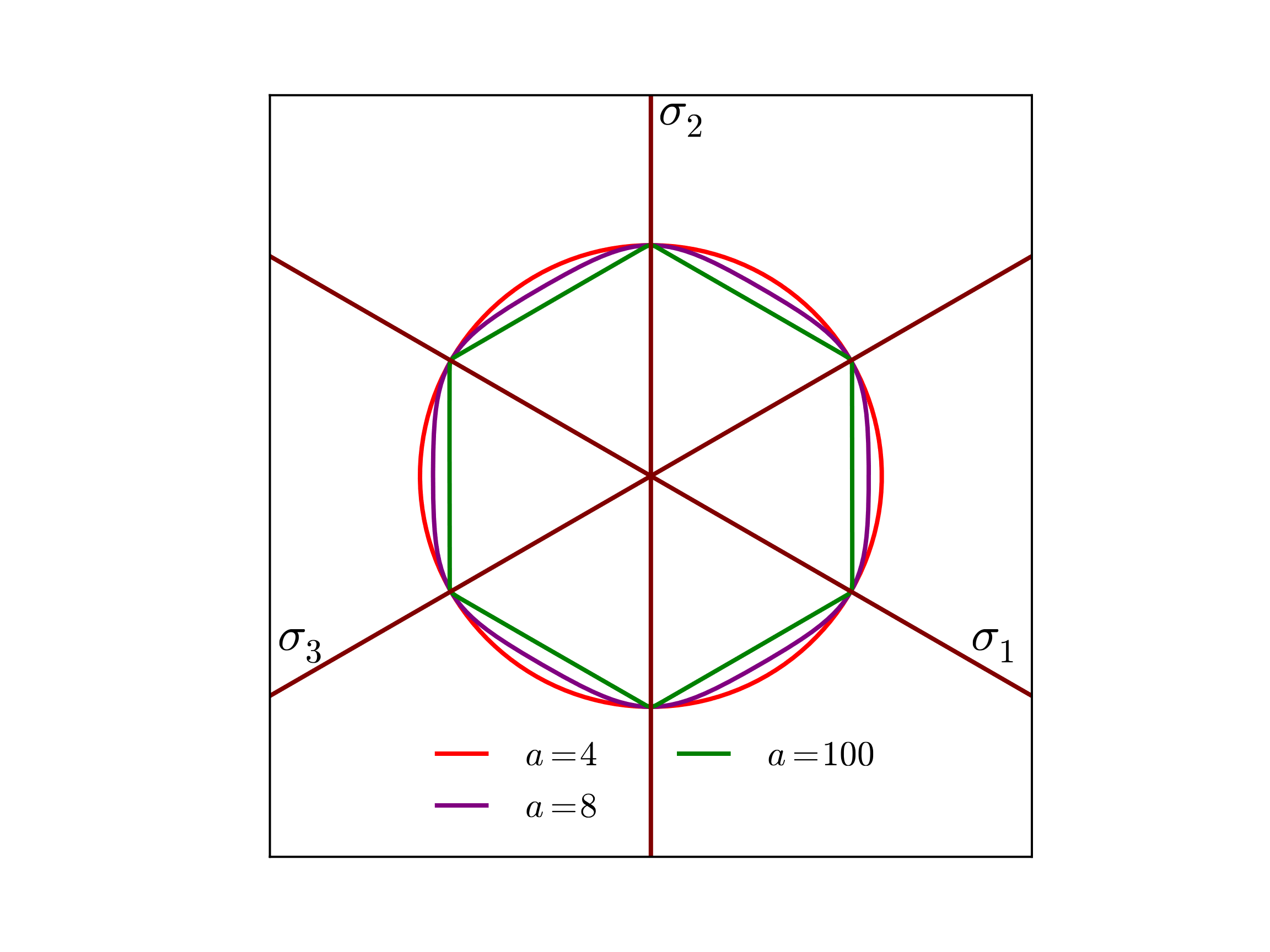
Fig. 5.7 Example Hosford yield surfaces, \(f\left(\sigma_{ij},\bar{\varepsilon}^p=0;a\right)\), presented in the deviatoric \(\pi\)-plane. The presented surfaces correspond to the different yield exponents \(a = 4, 8,\) and \(100\).
For the hardening function, \(\bar{\sigma}\left(\bar{\varepsilon}^p\right)\), a variety of forms including linear, power law, or a more general user defined function may be used.
An associated flow rule is utilized such that the plastic rate of deformation is normal to the yield surface and is given by,
where \(\dot{\gamma}\) is the consistency multiplier enforcing \(f=0\) during plastic deformation. Given the form of \(f\), it can also be shown that \(\dot{\gamma}=\dot{\bar{\varepsilon}}^p\).
For details on the plasticity model, please see [[15]]. Additional details on failure models and adiabatic heating capabilities may be found in [[10], [11]] and [[12]], respectively.
In the command blocks that define the Hosford plasticity model:
See Section 5.1.5 for more information on elastic constants input.
The reference nominal yield stress, \(\bar{\sigma}\), is defined with the
YIELD STRESScommand line.The yield surface exponent, \(a\), is defined with the
Acommand line.The type of hardening law is defined with the
HARDENING MODELcommand line, other hardening commands then define the specific shape of that hardening curve.The hardening modulus for a linear hardening model is defined with the
HARDENING MODULUScommand line.The hardening constant for a power law hardening model is defined with the
HARDENING CONSTANTcommand line.The hardening exponent for a power law hardening model is defined with the
HARDENING EXPONENTcommand line.The L"{u}ders strain for a power law hardening model is defined with the
LUDERS STRAINcommand line.The hardening function for a user defined hardening model is defined with the
HARDENING FUNCTIONcommand line.The shape of the spline for the spline based hardening is defined by the
CUBIC SPLINE TYPE,CARDINAL PARAMETER,KNOT EQPS, andKNOT STRESScommand lines.
Output variables available for this model are listed in Table 5.12.
Name |
Description |
|---|---|
|
equivalent plastic strain, \(\bar{\varepsilon}^{p}\) |
|
equivalent plastic strain rate, \(\dot{\bar{\varepsilon}}^{p}\) |
|
effective stress, \(\phi\) |
|
tensile equivalent plastic strain, \(\bar{\varepsilon}^{p}_{t}\) |
|
damage, \(\phi\) |
|
void count, \(\eta\) |
|
void size, \(\upsilon\) |
|
damage rate, \(\dot{\phi}\) |
|
void count rate, \(\dot{\eta}\) |
|
plastic work heat rate, \(\dot{Q}^p\) |
5.2.15. Hill Plasticity Model
BEGIN PARAMETERS FOR MODEL HILL_PLASTICITY
  #
  # Elastic constants
  #
  YOUNGS MODULUS = <real>
  POISSONS RATIO = <real>
  SHEAR MODULUS  = <real>
  BULK MODULUS   = <real>
  LAMBDA         = <real>
  TWO MU         = <real>
  #
  # Material coordinates system definition
  #
  COORDINATE SYSTEM             = <string> coordinate_system_name
  DIRECTION FOR ROTATION        = <real> 1|2|3
  ALPHA                         = <real> (degrees)
  SECOND DIRECTION FOR ROTATION = <real> 1|2|3
  SECOND ALPHA                  = <real> (degrees)
  #
  # Yield surface parameters
  #
  YIELD STRESS = <real>
  R11 = <real> (1.0)
  R22 = <real> (1.0)
  R33 = <real> (1.0)
  R12 = <real> (1.0)
  R23 = <real> (1.0)
  R31 = <real> (1.0)
  #
  # Hardening model
  #
  HARDENING MODEL = LINEAR | POWER_LAW | VOCE | USER_DEFINED |
    FLOW_STRESS | DECOUPLED_FLOW_STRESS | JOHNSON_COOK |
    POWER_LAW_BREAKDOWN
  #
  # Linear hardening
  #
  HARDENING MODULUS = <real>
  #
  # Power-law hardening
  #
  HARDENING CONSTANT = <real>
  HARDENING EXPONENT = <real> (0.5)
  LUDERS STRAIN      = <real> (0.0)
  #
  # Voce hardening
  #
  HARDENING MODULUS       = <real>
  EXPONENTIAL COEFFICIENT = <real>
  #
  # Johnson-Cook hardening
  #
  HARDENING FUNCTION = <string>hardening_function_name
  RATE CONSTANT      = <real>
  REFERENCE RATE     = <real>
  #
  # Power law breakdown hardening
  #
  HARDENING FUNCTION = <string>hardening_function_name
  RATE COEFFICIENT   = <real>
  RATE EXPONENT      = <real>
  # User defined hardening
  #
  HARDENING FUNCTION = <string>hardening_function_name
  #
  #
  # Following Commands Pertain to Flow_Stress Hardening Model
  #
  #    -  Isotropic Hardening model
  #
  ISOTROPIC HARDENING MODEL = LINEAR | POWER_LAW | VOCE |
                              USER_DEFINED
  #
  # Specifications for Linear, Power-law, and Voce same as above
  #
  # User defined hardening
  #
  ISOTROPIC HARDENING FUNCTION = <string>iso_hardening_fun_name
  #
  #     - Rate dependence
  #
  RATE MULTIPLIER = JOHNSON_COOK | POWER_LAW_BREAKDOWN |
     USER_DEFINED | RATE_INDEPENDENT (RATE_INDEPENDENT)
  #
  # Specifications for Johnson-Cook, Power-law-breakdown
  #     same as before EXCEPT no need to specify a
  #     hardening function
  #
  # User defined rate multiplier
  #
  RATE MULTIPLIER FUNCTION = <string> rate_mult_function_name
  #
  #     - Temperature dependence
  #
  TEMPERATURE MULTIPLIER = JOHNSON_COOK | USER_DEFINED |
     TEMPERATURE_INDEPENDENT (TEMPERATURE_INDEPENDENT)
  #
  #  Johnson-Cook temperature dependence
  #
  MELTING TEMPERATURE   = <real>
  REFERENCE TEMPERATURE = <real>
  TEMPERATURE EXPONENT  = <real>
  #
  #  User-defined temperature dependence
  TEMPERATURE MULTIPLIER FUNCTION = <string>temp_mult_function_name
  #
  # Following Commands Pertain to Decoupled_Flow_Stress Hardening Model
  #
  #    -  Isotropic Hardening model
  #
  ISOTROPIC HARDENING MODEL = LINEAR | POWER_LAW | VOCE | USER_DEFINED
  #
  # Specifications for Linear, Power-law, and Voce same as above
  #
  # User defined hardening
  #
  ISOTROPIC HARDENING FUNCTION = <string>isotropic_hardening_function_name
  #
  #     - Rate dependence
  #
  YIELD RATE MULTIPLIER = JOHNSON_COOK | POWER_LAW_BREAKDOWN |
              USER_DEFINED | RATE_INDEPENDENT (RATE_INDEPENDENT)
  #
  # Specifications for Johnson-Cook, Power-law-breakdown same as before
  #     EXCEPT no need to specify a hardening function
  #     AND should be preceded by YIELD
  #
  #     As an example for Johnson-Cook yield rate dependence,
  #
  YIELD RATE CONSTANT  = <real>
  YIELD REFERENCE RATE = <real>
  #
  # User defined rate multiplier
  #
  YIELD RATE MULTIPLIER FUNCTION = <string>yield_rate_mult_function_name
  #
  HARDENING_RATE MULTIPLIER = JOHNSON_COOK | POWER_LAW_BREAKDOWN |
              USER_DEFINED | RATE_INDEPENDENT (RATE_INDEPENDENT)
  #
  #     Syntax same as for yield parameters but with a HARDENING prefix
  #
  #     - Temperature dependence
  #
  YIELD TEMPERATURE MULTIPLIER = JOHNSON_COOK | USER_DEFINED |
            TEMPERATURE_INDEPENDENT (TEMPERATURE_INDEPENDENT)
  #
  #  Johnson-Cook temperature dependence
  #
  YIELD MELTING TEMPERATURE   = <real>
  YIELD REFERENCE TEMPERATURE = <real>
  YIELD TEMPERATURE EXPONENT  = <real>
  #
  #  User-defined temperature dependence
  YIELD TEMPERATURE MULTIPLIER FUNCTION = <string>yield_temp_mult_fun_name
  #
  HARDENING TEMPERATURE MULTIPLIER = JOHNSON_COOK | USER_DEFINED |
            TEMPERATURE_INDEPENDENT (TEMPERATURE_INDEPENDENT)
  #
  #   Syntax for hardening constants same as for yield but
  #            with HARDENING prefix
  #
  # Optional Failure Definitions
  #    Following only need to be defined if intend to use failure model
  #
  FAILURE MODEL = TEARING_PARAMETER | JOHNSON_COOK_FAILURE | WILKINS
                  | MODULAR_FAILURE | MODULAR_BCJ_FAILURE

  CRITICAL FAILURE PARAMETER = <real>
  #
  # TEARING_PARAMETER Failure model definitions
  #
  TEARING PARAMETER EXPONENT = <real>
  #
  # JOHNSON_COOK_FAILURE Failure model definitions
  #
  JOHNSON COOK D1       = <real>
  JOHNSON COOK D2       = <real>
  JOHNSON COOK D3       = <real>
  JOHNSON COOK D4       = <real>
  JOHNSON COOK D5       = <real>
  #
  #Following Johnson-Cook parameters can only be defined once.  As such, only
  #  needed if not previously defined via Johnson-Cook multipliers
  #  w/ flow-stress hardening.  Does need to be defined
  #  w/ Decoupled Flow Stress
  #
  REFERENCE RATE        = <real>
  REFERENCE TEMPERATURE = <real>
  MELTING TEMPERATURE   = <real>
  #
  # WILKINS Failure model definitions
  #
  WILKINS ALPHA    = <real>
  WILKINS BETA     = <real>
  WILKINS PRESSURE = <real>
  #
  #  MODULAR_FAILURE Failure model definitions
  #
  PRESSURE MULTIPLIER         = PRESSURE_INDEPENDENT | WILKINS
                                | USER_DEFINED (PRESSURE_INDEPENDENT)
  LODE ANGLE MULTIPLIER       = LODE_ANGLE_INDEPENDENT |
                                WILKINS (LODE_ANGLE_INDEPENDENT)
  TRIAXIALITY MULTIPLIER      = TRIAXIALITY_INDEPENDENT | JOHNSON_COOK
                                | USER_DEFINED (TRIAXIALITY_INDEPENDENT)
  RATE FAIL MULTIPLIER        = RATE_INDEPENDENT | JOHNSON_COOK
                                | USER_DEFINED (RATE_INDEPENDENT)
  TEMPERATURE FAIL MULTIPLIER = TEMPERATURE_INDEPENDENT | JOHNSON_COOK
                                | USER_DEFINED (TEMPERATURE_INDEPENDENT)
  #
  # Individual multiplier definitions
  #
  PRESSURE MULTIPLIER = WILKINS
  WILKINS ALPHA       = <real>
  WILKINS PRESSURE    = <real>
  #
  PRESSURE MULTIPLIER = USER_DEFINED
  PRESSURE MULTIPLIER FUNCTION = <string> pressure_multiplier_fun_name
  #
  LODE ANGLE MULTIPLIER = WILKINS
  WILKINS BETA          = <real>
  #
  TRIAXIALITY MULTIPLIER = JOHNSON_COOK
  JOHNSON COOK D1        = <real>
  JOHNSON COOK D2        = <real>
  JOHNSON COOK D3        = <real>
  #
  TRIAXIALITY MULTIPLIER = USER_DEFINED
  TRIAXIALITY MULTIPLIER FUNCTION = <string> triaxiality_multiplier_fun_name
  #
  RATE FAIL MULTIPLIER = JOHNSON_COOK
  JOHNSON COOK D4      = <real>
  # REFERENCE RATE should only be added if not previously defined
  REFERENCE RATE       = <real>
  #
  RATE FAIL MULTIPLIER = USER_DEFINED
  RATE FAIL MULTIPLIER FUNCTION = <string> rate_fail_multiplier_fun_name
  #
  TEMPERATURE FAIL MULTIPLIER = JOHNSON_COOK
  JOHNSON COOK D5             = <real>
  # JC Temperatures should only be defined if not previously given
  REFERENCE TEMPERATURE       = <real>
  MELTING TEMPERATURE         = <real>
  #
  TEMPERATURE FAIL MULTIPLIER          = USER_DEFINED
  TEMPERATURE FAIL MULTIPLIER FUNCTION = <string> temp_multiplier_fun_name
  #
  # MODULAR BCJ_FAILURE Failure model definitions
  #
  INITIAL DAMAGE    = <real>
  INITIAL VOID SIZE = <real>
  DAMAGE BETA       = <real> (0.5)
  GROWTH MODEL      = COCKS_ASHBY | NO_GROWTH (NO_GROWTH)
  NUCLEATION MODEL  = HORSTEMEYER_GOKHALE | CHU_NEEDLEMAN_STRAIN
                      | NO_NUCLEATION (NO_NUCLEATION)
  #
  GROWTH RATE FAIL MULTIPLIER        = JOHNSON_COOK | USER_DEFINED
                                       | RATE_INDEPENDENT
                                       (RATE_INDEPENDENT)
  GROWTH TEMPERATURE FAIL MULTIPLIER = JOHNSON_COOK | USER_DEFINED
                                       | TEMPERATURE_INDEPENDENT
                                       (TEMPERATURE_INDEPENDENT)
  #
  NUCLEATION RATE FAIL MULTIPLIER        = JOHNSON_COOK | USER_DEFINED
                                           | RATE_INDEPENDENT
                                           (RATE_INDEPENDENT)
  NUCLEATION TEMPERATURE FAIL MULTIPLIER = JOHNSON_COOK | USER_DEFINED
                                           | TEMPERATURE_INDEPENDENT
                                           (TEMPERATURE_INDEPENDENT)
  #
  # Definitions for individual growth and nucleation models
  #
  GROWTH MODEL = COCKS_ASHBY
  DAMAGE EXPONENT = <real> (0.5)
  #
  NUCLEATION MODEL      = HORSTEMEYER_GOKHALE
  NUCLEATION PARAMETER1 = <real> (0.0)
  NUCLEATION PARAMETER2 = <real> (0.0)
  NUCLEATION PARAMETER3 = <real> (0.0)
  #
  NUCLEATION MODEL          = CHU_NEEDLEMAN_STRAIN
  NUCLEATION AMPLITUDE      = <real>
  MEAN NUCLEATION STRAIN    = <real>
  NUCLEATION STRAIN STD DEV = <real>
  #
  # Definitions for rate and temperature fail multiplier
  #   Note: only showing definitions for growth.
  #    Nucleation terms are the same just with NUCLEATION instead
  #    of GROWTH
  #
  GROWTH RATE FAIL MULTIPLIER = JOHNSON_COOK
  GROWTH JOHNSON COOK D4      = <real>
  GROWTH REFERENCE RATE       = <real>
  #
  GROWTH RATE FAIL MULTIPLIER          = USER_DEFINED
  GROWTH RATE FAIL MULTIPLIER FUNCTION = <string> growth_rate_fail_mult_func
  #
  GROWTH TEMPERATURE FAIL MULTIPLIER = JOHNSON_COOK
  GROWTH JOHNSON COOK D5             = <real>
  GROWTH REFERENCE TEMPERATURE       = <real>
  GROWTH MELTING TEMPERATURE         = <real>
  #
  GROWTH TEMPERATURE FAIL MULTIPLIER          = USER_DEFINED
  GROWTH TEMPERATURE FAIL MULTIPLIER FUNCTION = <string> temp_fail_mult_func
  #
  #
  # Optional Adiabatic Heating/Thermal Softening  Definitions
  #    Following only need to be defined if intend to use failure model
  #
  THERMAL SOFTENING MODEL = ADIABATIC | COUPLED
  #
  SPECIFIC HEAT = <real> #not needed for COUPLED
  BETA_TQ       = <real>
END [PARAMETERS FOR MODEL HILL_PLASTICITY]
The Hill plasticity model is similar to other plasticity models except that it is not isotropic. It is a hypoelastic, rate-independent plasticity model. The rate form of the equation assumes an additive split of the rate of deformation into an elastic and plastic part
The stress rate only depends on the elastic rate of deformation
where \(\mathbb{C}_{ijkl}\) are the components of the fourth-order, isotropic elasticity tensor.
The Hill plasticity model has an orthotropic yield surface that assumes orthogonal principal material directions. An example of this yield surface is presented below in Fig. 5.8 along with examples of two isotropic surfaces – the von Mises (\(J_2\)) and Hosford (with \(a=8\)). The various surface parameters correspond to 2090-T3 aluminum and the specific Hill strengths are found in [[15]]. By comparing the Hill surface to the two isotropic surfaces, the impact of the anisotropy is clear. Additionally, substantial differences to the normals of the yield surfaces at points of intersection highlight the impact of the yield function selection on the resulting flow directions.
Like other plasticity models, the Hill yield surface, \(f\), is written,
with \(\phi\) being the effective stress and \(\bar{\sigma}\) is the current yield stress that may be dependent on rate and/or temperature. The Hill effective stress is essentially an orthotropic extension of the von Mises function. After accounting for plastic incompressibility and related constraints, there are six individual yield stresses: \(\sigma^{y}_{11}\), \(\sigma^{y}_{22}\), \(\sigma^{y}_{33}\), \(\tau^{y}_{12}\), \(\tau^{y}_{23}\), and \(\tau^{y}_{31}\). These yield stresses correspond to 3 normal and 3 shear yield stresses. Written in terms of the components, the effective stress has the form,
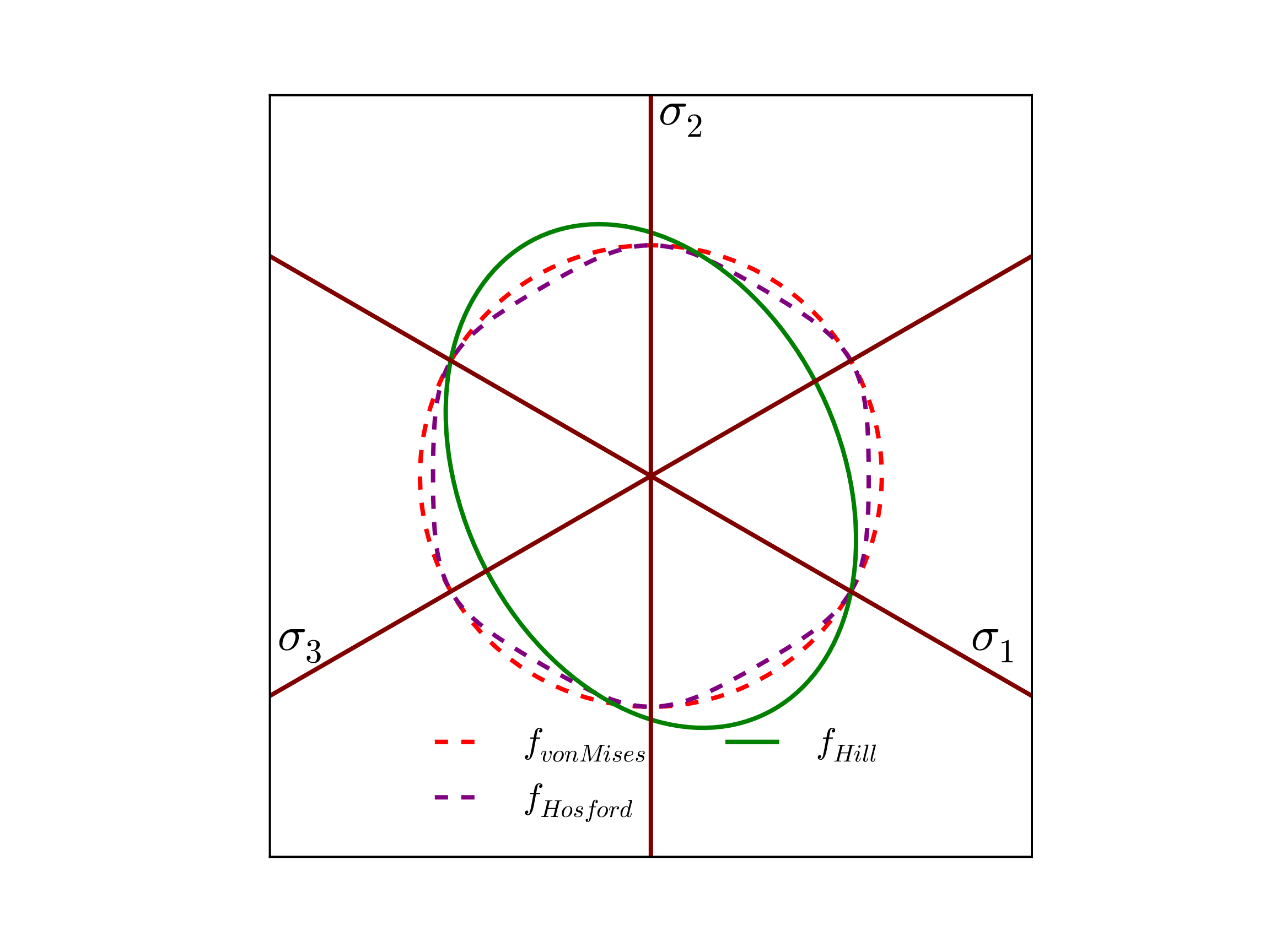
Fig. 5.8 Example anisotropic Hill yield surface, \(f_{Hill}\left(\sigma_{ij},\bar{\varepsilon}^p=0\right)\), presented in the deviatoric \(\pi\)-plane fit to 2090-T3 aluminum. Comparison von Mises (\(J_2\)) and Hosford (with \(a=8\)) surfaces are also presented.
The coefficients \(F\), \(G\), \(H\), \(L\), \(M\), and \(N\) were introduced by Hill. In terms of the yield stresses they are:
where \(\bar{\sigma}\) is a reference yield stress.
Rather than input the six independent yield stresses, the ratios of the yield stresses to some reference yield stress are generally used as input. These ratios are
These ratios are set up so that if \(R_{ij} = 1\) then the yield surface is isotropic.
The orientation of the principal material axes with respect to the global Cartesian axes may be specified by the user. First, a rectangular or cylindrical reference coordinate system is defined. Spherical coordinate systems are not currently implemented for the Hill model. The material coordinate system can then be defined through two successive rotations about axes in the reference rectangular or cylindrical coordinate system. In the case of the cylindrical coordinate system this allows the principal material axes to vary point-wise in a given element block. Refer to Section 5.1.7 for details on the definition of material coordinate systems.
The plastic rate of deformation, as with the isotropic models, assumes associated flow
Given the form for \(\phi\), the consistency parameter, \(\dot\gamma\) is equal to the rate of the equivalent plastic strain, \(\dot{\bar{\varepsilon}}^{p}\).
For more information about the Hill plasticity model, consult [[16]]. Additional discussion on options for failure models and adiabatic heating may be found in [[10], [11]] and [[12]], respectively.
In the command blocks that define the Hill plasticity model:
See Section 5.1.5 for more information on elastic constants input.
See Section 5.1.7 for more information on material coordinates system definition commands.
The reference nominal yield stress, \(\bar{\sigma}\), is defined with the
YIELD STRESScommand line.The ratio of the normal yield stress in the \(\bar{\bf e}_{1}\bar{\bf e}_{1}\) material direction is defined with the
R11command line. The default is 1.0.The ratio of the normal yield stress in the \(\bar{\bf e}_{2}\bar{\bf e}_{2}\) material direction is defined with the
R22command line. The default is 1.0.The ratio of the normal yield stress in the \(\bar{\bf e}_{3}\bar{\bf e}_{3}\) material direction is defined with the
R33command line. The default is 1.0.The ratio of the shear yield stress in the \(\bar{\bf e}_{1}\bar{\bf e}_{2}\) material direction is defined with the
R12command line. The default is 1.0.The ratio of the shear yield stress in the \(\bar{\bf e}_{2}\bar{\bf e}_{3}\) material direction is defined with the
R23command line. The default is 1.0.The ratio of the shear yield stress in the \(\bar{\bf e}_{3}\bar{\bf e}_{1}\) material direction is defined with the
R31command line. The default is 1.0.The type of hardening law is defined with the
HARDENING MODELcommand line, other hardening commands then define the specific shape of that hardening curve.The hardening modulus for a linear hardening model is defined with the
HARDENING MODULUScommand line.The hardening constant for a power law hardening model is defined with the
HARDENING CONSTANTcommand line.The hardening exponent for a power law hardening model is defined with the
HARDENING EXPONENTcommand line.The L"{u}ders strain for a power law hardening model is defined with the
LUDERS STRAINcommand line.The hardening function for a user defined hardening model is defined with the
HARDENING FUNCTIONcommand line.The shape of the spline for the spline based hardening is defined by the
CUBIC SPLINE TYPE,CARDINAL PARAMETER,KNOT EQPS, andKNOT STRESScommand lines.
Output variables available for this model are listed in Table 5.13.
Name |
Description |
|---|---|
|
equivalent plastic strain, \(\bar{\varepsilon}^{p}\) |
|
equivalent plastic strain rate, \(\dot{\bar{\varepsilon}}^{p}\) |
|
effective stress, \(\phi\) |
|
tensile equivalent plastic strain, \(\bar{\varepsilon}^{p}_{t}\) |
|
damage, \(\phi\) |
|
void count, \(\eta\) |
|
void size, \(\upsilon\) |
|
damage rate, \(\dot{\phi}\) |
|
void count rate, \(\dot{\eta}\) |
|
plastic work heat rate, \(\dot{Q}^p\) |
5.2.16. Barlat Plasticity Model
BEGIN PARAMETERS FOR MODEL BARLAT_PLASTICITY
  #
  # Elastic constants
  #
  YOUNGS MODULUS = <real>
  POISSONS RATIO = <real>
  SHEAR MODULUS  = <real>
  BULK MODULUS   = <real>
  LAMBDA         = <real>
  TWO MU         = <real>
  #
  # Material coordinates system definition
  #
  COORDINATE SYSTEM             = <string> coordinate_system_name
  DIRECTION FOR ROTATION        = <real> 1|2|3
  ALPHA                         = <real> (degrees)
  SECOND DIRECTION FOR ROTATION = <real> 1|2|3
  SECOND ALPHA                  = <real> (degrees)
  #
  # Yield surface parameters
  #
  YIELD STRESS = <real>
  A            = <real> (4.0)
  CP12         = <real> (1.0)
  CP13         = <real> (1.0)
  CP21         = <real> (1.0)
  CP23         = <real> (1.0)
  CP31         = <real> (1.0)
  CP32         = <real> (1.0)
  CP44         = <real> (1.0)
  CP55         = <real> (1.0)
  CP66         = <real> (1.0)
  CPP12        = <real> (1.0)
  CPP13        = <real> (1.0)
  CPP21        = <real> (1.0)
  CPP23        = <real> (1.0)
  CPP31        = <real> (1.0)
  CPP32        = <real> (1.0)
  CPP44        = <real> (1.0)
  CPP55        = <real> (1.0)
  CPP66        = <real> (1.0)
  #
  # Hardening model
  #
  HARDENING MODEL = LINEAR | POWER_LAW | VOCE | USER_DEFINED |
    FLOW_STRESS | DECOUPLED_FLOW_STRESS | JOHNSON_COOK |
    POWER_LAW_BREAKDOWN
  #
  # Linear hardening
  #
  HARDENING MODULUS = <real>
  #
  # Power-law hardening
  #
  HARDENING CONSTANT = <real>
  HARDENING EXPONENT = <real> (0.5)
  LUDERS STRAIN      = <real> (0.0)
  #
  # Voce hardening
  #
  HARDENING MODULUS       = <real>
  EXPONENTIAL COEFFICIENT = <real>
  #
  # Johnson-Cook hardening
  #
  HARDENING FUNCTION = <string>hardening_function_name
  RATE CONSTANT      = <real>
  REFERENCE RATE     = <real>
  #
  # Power law breakdown hardening
  #
  HARDENING FUNCTION = <string>hardening_function_name
  RATE COEFFICIENT   = <real>
  RATE EXPONENT      = <real>
  # User defined hardening
  #
  HARDENING FUNCTION = <string>hardening_function_name
  #
  #
  # Following Commands Pertain to Flow_Stress Hardening Model
  #
  #    -  Isotropic Hardening model
  #
  ISOTROPIC HARDENING MODEL = LINEAR | POWER_LAW | VOCE |
                              USER_DEFINED
  #
  # Specifications for Linear, Power-law, and Voce same as above
  #
  # User defined hardening
  #
  ISOTROPIC HARDENING FUNCTION = <string>iso_hardening_fun_name
  #
  #     - Rate dependence
  #
  RATE MULTIPLIER = JOHNSON_COOK | POWER_LAW_BREAKDOWN |
     USER_DEFINED | RATE_INDEPENDENT (RATE_INDEPENDENT)
  #
  # Specifications for Johnson-Cook, Power-law-breakdown
  #     same as before EXCEPT no need to specify a
  #     hardening function
  #
  # User defined rate multiplier
  #
  RATE MULTIPLIER FUNCTION = <string> rate_mult_function_name
  #
  #     - Temperature dependence
  #
  TEMPERATURE MULTIPLIER = JOHNSON_COOK | USER_DEFINED |
     TEMPERATURE_INDEPENDENT (TEMPERATURE_INDEPENDENT)
  #
  #  Johnson-Cook temperature dependence
  #
  MELTING TEMPERATURE   = <real>
  REFERENCE TEMPERATURE = <real>
  TEMPERATURE EXPONENT  = <real>
  #
  #  User-defined temperature dependence
  TEMPERATURE MULTIPLIER FUNCTION = <string>temp_mult_function_name
  #
  # Following Commands Pertain to Decoupled_Flow_Stress Hardening Model
  #
  #    -  Isotropic Hardening model
  #
  ISOTROPIC HARDENING MODEL = LINEAR | POWER_LAW | VOCE | USER_DEFINED
  #
  # Specifications for Linear, Power-law, and Voce same as above
  #
  # User defined hardening
  #
  ISOTROPIC HARDENING FUNCTION = <string>isotropic_hardening_function_name
  #
  #     - Rate dependence
  #
  YIELD RATE MULTIPLIER = JOHNSON_COOK | POWER_LAW_BREAKDOWN |
              USER_DEFINED | RATE_INDEPENDENT (RATE_INDEPENDENT)
  #
  # Specifications for Johnson-Cook, Power-law-breakdown same as before
  #     EXCEPT no need to specify a hardening function
  #     AND should be preceded by YIELD
  #
  #     As an example for Johnson-Cook yield rate dependence,
  #
  YIELD RATE CONSTANT  = <real>
  YIELD REFERENCE RATE = <real>
  #
  # User defined rate multiplier
  #
  YIELD RATE MULTIPLIER FUNCTION = <string>yield_rate_mult_function_name
  #
  HARDENING_RATE MULTIPLIER = JOHNSON_COOK | POWER_LAW_BREAKDOWN |
              USER_DEFINED | RATE_INDEPENDENT (RATE_INDEPENDENT)
  #
  #     Syntax same as for yield parameters but with a HARDENING prefix
  #
  #     - Temperature dependence
  #
  YIELD TEMPERATURE MULTIPLIER = JOHNSON_COOK | USER_DEFINED |
            TEMPERATURE_INDEPENDENT (TEMPERATURE_INDEPENDENT)
  #
  #  Johnson-Cook temperature dependence
  #
  YIELD MELTING TEMPERATURE   = <real>
  YIELD REFERENCE TEMPERATURE = <real>
  YIELD TEMPERATURE EXPONENT  = <real>
  #
  #  User-defined temperature dependence
  YIELD TEMPERATURE MULTIPLIER FUNCTION = <string>yield_temp_mult_fun_name
  #
  HARDENING TEMPERATURE MULTIPLIER = JOHNSON_COOK | USER_DEFINED |
            TEMPERATURE_INDEPENDENT (TEMPERATURE_INDEPENDENT)
  #
  #   Syntax for hardening constants same as for yield but
  #            with HARDENING prefix
  #
  # Optional Failure Definitions
  #    Following only need to be defined if intend to use failure model
  #
  FAILURE MODEL = TEARING_PARAMETER | JOHNSON_COOK_FAILURE | WILKINS
                  | MODULAR_FAILURE | MODULAR_BCJ_FAILURE

  CRITICAL FAILURE PARAMETER = <real>
  #
  # TEARING_PARAMETER Failure model definitions
  #
  TEARING PARAMETER EXPONENT = <real>
  #
  # JOHNSON_COOK_FAILURE Failure model definitions
  #
  JOHNSON COOK D1       = <real>
  JOHNSON COOK D2       = <real>
  JOHNSON COOK D3       = <real>
  JOHNSON COOK D4       = <real>
  JOHNSON COOK D5       = <real>
  #
  #Following Johnson-Cook parameters can only be defined once.  As such, only
  #  needed if not previously defined via Johnson-Cook multipliers
  #  w/ flow-stress hardening.  Does need to be defined
  #  w/ Decoupled Flow Stress
  #
  REFERENCE RATE        = <real>
  REFERENCE TEMPERATURE = <real>
  MELTING TEMPERATURE   = <real>
  #
  # WILKINS Failure model definitions
  #
  WILKINS ALPHA    = <real>
  WILKINS BETA     = <real>
  WILKINS PRESSURE = <real>
  #
  #  MODULAR_FAILURE Failure model definitions
  #
  PRESSURE MULTIPLIER         = PRESSURE_INDEPENDENT | WILKINS
                                | USER_DEFINED (PRESSURE_INDEPENDENT)
  LODE ANGLE MULTIPLIER       = LODE_ANGLE_INDEPENDENT |
                                WILKINS (LODE_ANGLE_INDEPENDENT)
  TRIAXIALITY MULTIPLIER      = TRIAXIALITY_INDEPENDENT | JOHNSON_COOK
                                | USER_DEFINED (TRIAXIALITY_INDEPENDENT)
  RATE FAIL MULTIPLIER        = RATE_INDEPENDENT | JOHNSON_COOK
                                | USER_DEFINED (RATE_INDEPENDENT)
  TEMPERATURE FAIL MULTIPLIER = TEMPERATURE_INDEPENDENT | JOHNSON_COOK
                                | USER_DEFINED (TEMPERATURE_INDEPENDENT)
  #
  # Individual multiplier definitions
  #
  PRESSURE MULTIPLIER = WILKINS
  WILKINS ALPHA       = <real>
  WILKINS PRESSURE    = <real>
  #
  PRESSURE MULTIPLIER = USER_DEFINED
  PRESSURE MULTIPLIER FUNCTION = <string> pressure_multiplier_fun_name
  #
  LODE ANGLE MULTIPLIER = WILKINS
  WILKINS BETA          = <real>
  #
  TRIAXIALITY MULTIPLIER = JOHNSON_COOK
  JOHNSON COOK D1        = <real>
  JOHNSON COOK D2        = <real>
  JOHNSON COOK D3        = <real>
  #
  TRIAXIALITY MULTIPLIER = USER_DEFINED
  TRIAXIALITY MULTIPLIER FUNCTION = <string> triaxiality_multiplier_fun_name
  #
  RATE FAIL MULTIPLIER = JOHNSON_COOK
  JOHNSON COOK D4      = <real>
  # REFERENCE RATE should only be added if not previously defined
  REFERENCE RATE       = <real>
  #
  RATE FAIL MULTIPLIER = USER_DEFINED
  RATE FAIL MULTIPLIER FUNCTION = <string> rate_fail_multiplier_fun_name
  #
  TEMPERATURE FAIL MULTIPLIER = JOHNSON_COOK
  JOHNSON COOK D5             = <real>
  # JC Temperatures should only be defined if not previously given
  REFERENCE TEMPERATURE       = <real>
  MELTING TEMPERATURE         = <real>
  #
  TEMPERATURE FAIL MULTIPLIER          = USER_DEFINED
  TEMPERATURE FAIL MULTIPLIER FUNCTION = <string> temp_multiplier_fun_name
  #
  # MODULAR BCJ_FAILURE Failure model definitions
  #
  INITIAL DAMAGE    = <real>
  INITIAL VOID SIZE = <real>
  DAMAGE BETA       = <real> (0.5)
  GROWTH MODEL      = COCKS_ASHBY | NO_GROWTH (NO_GROWTH)
  NUCLEATION MODEL  = HORSTEMEYER_GOKHALE | CHU_NEEDLEMAN_STRAIN
                      | NO_NUCLEATION (NO_NUCLEATION)
  #
  GROWTH RATE FAIL MULTIPLIER        = JOHNSON_COOK | USER_DEFINED
                                       | RATE_INDEPENDENT
                                       (RATE_INDEPENDENT)
  GROWTH TEMPERATURE FAIL MULTIPLIER = JOHNSON_COOK | USER_DEFINED
                                       | TEMPERATURE_INDEPENDENT
                                       (TEMPERATURE_INDEPENDENT)
  #
  NUCLEATION RATE FAIL MULTIPLIER        = JOHNSON_COOK | USER_DEFINED
                                           | RATE_INDEPENDENT
                                           (RATE_INDEPENDENT)
  NUCLEATION TEMPERATURE FAIL MULTIPLIER = JOHNSON_COOK | USER_DEFINED
                                           | TEMPERATURE_INDEPENDENT
                                           (TEMPERATURE_INDEPENDENT)
  #
  # Definitions for individual growth and nucleation models
  #
  GROWTH MODEL = COCKS_ASHBY
  DAMAGE EXPONENT = <real> (0.5)
  #
  NUCLEATION MODEL      = HORSTEMEYER_GOKHALE
  NUCLEATION PARAMETER1 = <real> (0.0)
  NUCLEATION PARAMETER2 = <real> (0.0)
  NUCLEATION PARAMETER3 = <real> (0.0)
  #
  NUCLEATION MODEL          = CHU_NEEDLEMAN_STRAIN
  NUCLEATION AMPLITUDE      = <real>
  MEAN NUCLEATION STRAIN    = <real>
  NUCLEATION STRAIN STD DEV = <real>
  #
  # Definitions for rate and temperature fail multiplier
  #   Note: only showing definitions for growth.
  #    Nucleation terms are the same just with NUCLEATION instead
  #    of GROWTH
  #
  GROWTH RATE FAIL MULTIPLIER = JOHNSON_COOK
  GROWTH JOHNSON COOK D4      = <real>
  GROWTH REFERENCE RATE       = <real>
  #
  GROWTH RATE FAIL MULTIPLIER          = USER_DEFINED
  GROWTH RATE FAIL MULTIPLIER FUNCTION = <string> growth_rate_fail_mult_func
  #
  GROWTH TEMPERATURE FAIL MULTIPLIER = JOHNSON_COOK
  GROWTH JOHNSON COOK D5             = <real>
  GROWTH REFERENCE TEMPERATURE       = <real>
  GROWTH MELTING TEMPERATURE         = <real>
  #
  GROWTH TEMPERATURE FAIL MULTIPLIER          = USER_DEFINED
  GROWTH TEMPERATURE FAIL MULTIPLIER FUNCTION = <string> temp_fail_mult_func
  #
  #
  # Optional Adiabatic Heating/Thermal Softening  Definitions
  #    Following only need to be defined if intend to use failure model
  #
  THERMAL SOFTENING MODEL = ADIABATIC | COUPLED
  #
  SPECIFIC HEAT = <real> #not needed for COUPLED
  BETA_TQ       = <real>
END [PARAMETERS FOR MODEL BARLAT_PLASTICITY]
The Barlat plasticity model is a hypoelastic, rate-independent plasticity model. The underlying yield surface is both anisotropic and non-quadratic [[17]]. With respect to the former, linear transformations of the deviatoric stress are used to capture texture and anisotropy effects. The rate form of this model assumes an additive split of the rate of deformation into an elastic and plastic part
The stress rate only depends on the elastic rate of deformation
where \(\mathbb{C}_{ijkl}\) are the components of the fourth-order, isotropic elasticity tensor.
To describe anisotropy in the yield-behavior, two linear transformation tensors, \(C^{\prime}_{ijkl}\) and \(C^{\prime\prime}_{ijkl}\), are introduced such that,
with \(s_{ij}\) being the deviatoric stress tensor (\(s_{ij}=\sigma_{ij}-1/3\sigma_{kk}\delta_{ij}\)) and \(s_{ij}^{\prime}\) and \(s_{ij}^{\prime\prime}\) being transformed stresses. Two transformations are used to capture both the anisotropy of the yield surface and flow rule. In Voigt notation the two transformation tensors are given as,
Alternatively, the transformed stresses may be written in terms of the Cauchy stress tensor as,
where \(L^{\prime}_{ijkl}=C^{\prime}_{ijmn}I\!I_{mnkl}\) and \(L^{\prime\prime}_{ijkl}=C^{\prime\prime}_{ijmn}I\!I_{mnkl}\). In this case, \(I\!I_{ijkl}\) is the symmetric deviatoric projection tensor and takes the form of,
In reduced form,
and an analogous expression may be written for \(L^{\prime\prime}_{ijkl}\).
The yield surface, \(f\), is given as,
in which \(\phi\left(\sigma_{ij}\right)\) is the effective stress and \(\bar{\sigma}\left(\bar{\varepsilon}^p\right)\) is the current yield stress that may depend on rate and/or temperature. The effective stress is written in terms of the principal transformed stresses (\(s^{\prime}_i\) and \(s^{\prime\prime}_i\),respectively) and the yield surface exponent, \(a\), as,
An example of such a yield surface is given in Fig. 5.9 along with examples of previously presented (von Mises, Hosford, Hill) surfaces. The presented Barlat surface corresponds to that of 2090-T3 aluminum first characterized by Barlat et al. [[17]]. In Fig. 5.9, both the anisotropy and non-quadratic nature of the yield surface is evident leading to differing strengths and flow directions at various stresses from any of the other models.
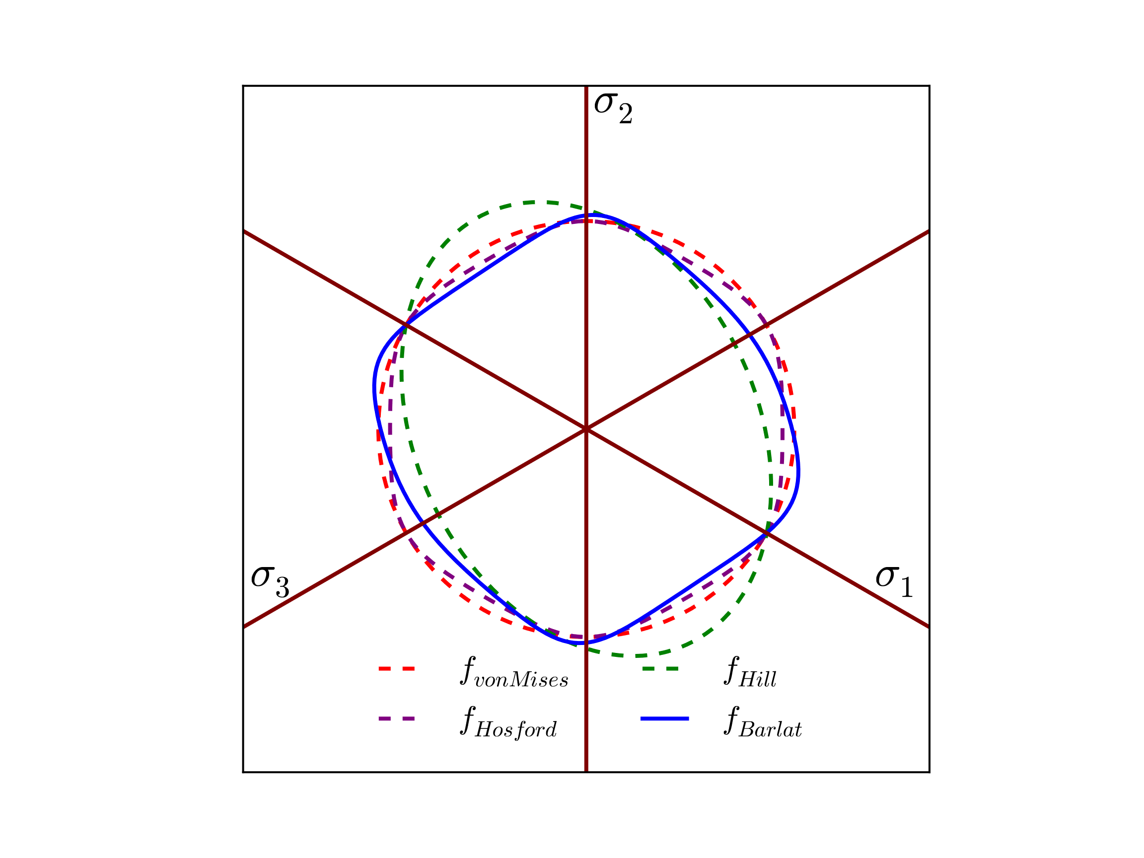
Fig. 5.9 Example Barlat yield surface, \(f_{Barlat}\left(\sigma_{ij},\bar{\varepsilon}^p=0\right)\), of 2090-T3 aluminum presented in the deviatoric \(\pi\)-plane. Comparison von Mises (\(J_2\)), Hosford (with \(a=8\)), and Hill surfaces are also presented for comparison.
The orientation of the principal material axes with respect to the global Cartesian axes may be specified by the user. First, a rectangular or cylindrical reference coordinate system is defined. Spherical coordinate systems are not currently implemented for the Barlat model. The material coordinate system can then be defined through two successive rotations about axes in the reference rectangular or cylindrical coordinate system. In the case of the cylindrical coordinate system this allows the principal material axes to vary point-wise in a given element block. Refer to Section 5.1.7 for details on the definition of material coordinate systems.
The plastic rate of deformation, as with the isotropic models, assumes associated flow
in which \(\dot{\gamma}\) is the consistency multiplier. Given the form for \(\phi\), \(\dot\gamma\) is equal to the rate of the equivalent plastic strain, \(\dot{\bar{\varepsilon}}^{p}\). As the yield surface is cast in transformed stress space, determining the flow direction in Cartesian space may be done via the chain rule (details may be found in [[15]]) leading to an expression of the form,
For more information about the Barlat plasticity model, consult [[17], [15]]. Additional discussion on options for failure models and adiabatic heating may be found in [[10], [11]] and [[12]], respectively.
In the command blocks that define the Barlat plasticity model:
See Section 5.1.5 for more information on elastic constants input.
See Section 5.1.7 for more information on material coordinates system definition commands.
The reference nominal yield stress, \(\bar{\sigma}\), is defined with the
YIELD STRESScommand line.The exponent for the yield surface description, \(a\), is defined with the
Acommand line.The transformation coefficient, \(c^{'}_{12}\), is defined with the
CP12command line. It is defaulted to 1.0.The transformation coefficient, \(c^{'}_{13}\), is defined with the
CP13command line. It is defaulted to 1.0.The transformation coefficient, \(c^{'}_{21}\), is defined with the
CP21command line. It is defaulted to 1.0.The transformation coefficient, \(c^{'}_{23}\), is defined with the
CP23command line. It is defaulted to 1.0.The transformation coefficient, \(c^{'}_{31}\), is defined with the
CP31command line. It is defaulted to 1.0.The transformation coefficient, \(c^{'}_{32}\), is defined with the
CP32command line. It is defaulted to 1.0.The transformation coefficient, \(c^{'}_{44}\), is defined with the
CP44command line. It is defaulted to 1.0.The transformation coefficient, \(c^{'}_{55}\), is defined with the
CP55command line. It is defaulted to 1.0.The transformation coefficient, \(c^{'}_{66}\), is defined with the
CP66command line. It is defaulted to 1.0.The transformation coefficient, \(c^{''}_{12}\), is defined with the
CPP12command line. It is defaulted to 1.0.The transformation coefficient, \(c^{''}_{13}\), is defined with the
CPP13command line. It is defaulted to 1.0.The transformation coefficient, \(c^{''}_{21}\), is defined with the
CPP21command line. It is defaulted to 1.0.The transformation coefficient, \(c^{''}_{23}\), is defined with the
CPP23command line. It is defaulted to 1.0.The transformation coefficient, \(c^{''}_{31}\), is defined with the
CPP31command line. It is defaulted to 1.0.The transformation coefficient, \(c^{''}_{32}\), is defined with the
CPP32command line. It is defaulted to 1.0.The transformation coefficient, \(c^{''}_{44}\), is defined with the
CPP44command line. It is defaulted to 1.0.The transformation coefficient, \(c^{''}_{55}\), is defined with the
CPP55command line. It is defaulted to 1.0.The transformation coefficient, \(c^{''}_{66}\), is defined with the
CPP66command line. It is defaulted to 1.0.The type of hardening law is defined with the
HARDENING MODELcommand line, other hardening commands then define the specific shape of that hardening curve.The hardening modulus for a linear hardening model is defined with the
HARDENING MODULUScommand line.The hardening constant for a power law hardening model is defined with the
HARDENING CONSTANTcommand line.The hardening exponent for a power law hardening model is defined with the
HARDENING EXPONENTcommand line.The L"{u}ders strain for a power law hardening model is defined with the
LUDERS STRAINcommand line.The hardening function for a user defined hardening model is defined with the
HARDENING FUNCTIONcommand line.The shape of the spline for the spline based hardening is defined by the
CUBIC SPLINE TYPE,CARDINAL PARAMETER,KNOT EQPS, andKNOT STRESScommand lines.
Output variables available for this model are listed in Table 5.14.
Name |
Description |
|---|---|
|
equivalent plastic strain, \(\bar{\varepsilon}^{p}\) |
|
equivalent plastic strain rate, \(\dot{\bar{\varepsilon}}^{p}\) |
|
effective stress, \(\phi\) |
|
tensile equivalent plastic strain, \(\bar{\varepsilon}^{p}_{t}\) |
|
damage, \(\phi\) |
|
void count, \(\eta\) |
|
void size, \(\upsilon\) |
|
damage rate, \(\dot{\phi}\) |
|
void count rate, \(\dot{\eta}\) |
|
plastic work heat rate, \(\dot{Q}^p\) |
5.2.17. Johnson–Cook Model
BEGIN PARAMETERS FOR MODEL JOHNSON_COOK
  #
  # Elastic constants
  #
  YOUNGS MODULUS = <real>
  POISSONS RATIO = <real>
  SHEAR MODULUS  = <real>
  BULK MODULUS   = <real>
  LAMBDA         = <real>
  TWO MU         = <real>
  #
  # Yield surface parameters
  #
  YIELD STRESS = <real>
  HARDENING CONSTANT = <real>hardening_constant
  HARDENING EXPONENT = <real>hardening_exponent
  RHOCV = <real>rho_cv
  RATE CONSTANT = <real>rate_constant
  REFERENCE RATE = <real>reference_rate(0.001)
  D1 = <real>d1(0.0)
  D2 = <real>d2(0.0)
  D3 = <real>d3(0.0)
  D4 = <real>d4(0.0)
  D5 = <real>d5(0.0)
  EDOT_REF = <real>edot_ref(0.0)
  #
  # Temperature softening commands
  #
  BETA = <real>beta(0.95)
  THERMAL EXPONENT = <real>thermal_exponent
  REFERENCE TEMPERATURE = <real>reference_temperature
  MELT TEMPERATURE = <real>melt_temperature
  INITIAL TEMPERATURE = <real>init_temperature
  FORMULATION = <int>form(0)
END [PARAMETERS FOR MODEL JOHNSON_COOK]
The Johnson–Cook model is used to model materials—typically metals—undergoing plastic deformation at high rates and finite strains. The hardening function is rate- and temperature-dependent and is defined by
where \(\sigma_y\) is the yield stress, \(B\) is the hardening constant, \(\bar{\varepsilon}_p\) is the equivalent plastic strain, \(N\) is the hardening exponent, and \(C\) is the rate constant. The non-dimensional effective total strain rate \(\dot\varepsilon^{*}\) is given by
where \(\dot{\varepsilon}_{0}\) is a reference strain rate defined by the input EDOT_REF material parameter. Note if EDOT_REF is undefined, then \(\dot{\varepsilon}^{*}\) is set to the larger of either the maximum strain rate the material has encountered or the REFERENCE RATE input parameter. If EDOT_REF is defined, then the REFERENCE RATE input is not used by the model and has no effect. The Macaulay brackets in (5.25) ensure that \(\sigma\) is equal to the static flow stress \(\sigma_{\text{s}} = \left[ \sigma_y + B \left(\bar{\varepsilon}_p\right)^{N} \right]\left[ 1 - \theta^{*\,M} \right]\) when \(\dot{\varepsilon}<\dot{\varepsilon}_{0}\).
Parameter \(T^{*}\) is the homologous temperature and is defined as
where \(T\) is the current temperature, \(T_{ref}\) is the reference temperature, and \(T_{melt}\) is the melt temperature. In the case where \(M \le 0\), \((1-(T^{*})^{M}) = 1\).
Note that the temperature used internal to the Johnson–Cook model is not the standard model “temperature” field. Instead, the material temperature is defined via the INITIAL TEMPERATURE command. Plastic work internal to the model results in adiabatic heating and raises the material temperature. The resulting change in temperature is computed according to
where \(\rho\) is the material density, \(C_v\) is the specific heat, and \(\beta\) is the fraction of plastic work that is converted to heat, where \(0 \le \beta \le 1\). By default, \(\beta = 0.95\) though it may be set to a different value with the BETA command.
The Johnson–Cook model also encapsulates a failure criterion; the damage model [[9]] has a failure strain given by
where \(D_{1}\), \(D_{2}\), \(D_{3}\), \(D_{4}\), and \(D_{5}\) are material parameters, \(\sigma^{*}\) is the triaxiality, \(\sigma^{*} = \sigma_{m}/\bar{\sigma}\), \(\dot{\varepsilon}^{*}\) is the dimensionless strain rate, and \(T^{*}\) is the homologous temperature, both defined above. Damage is accumulated over time:
When \(D=1\), the material has failed. By default, fracture behavior is not active. For more information about the Johnson–Cook material model, consult [[8], [9]].
5.2.17.1. Command lines
Valid command lines for a command block defining a Johnson–Cook model are as follows:
Elastic constants: Consult Section 5.1.5 for information on elastic constants input.
YIELD STRESSdefines \(\sigma_{y}\), the stress for onset of yield and plasticity.HARDENING CONSTANTdefines \(B\).HARDENING EXPONENTdefines \(N\).RHOCVdefines \({\rho}C_v\), the volumetric heat capacity.INITIAL TEMPERATUREdefines the material initial temperature. Note that the Johnson–Cook material model temperature is not linked to the standard model “temperature” field that is set fromBEGIN PRESCRIBED TEMPERATUREcommand blocks.THERMAL EXPONENTdefines the thermal exponent \(M\).REFERENCE TEMPERATUREdefines the reference temperature \(T_{ref}\).MELT TEMPERATUREdefines the melt temperature \(T_{melt}\).REFERENCE RATEdefines the reference strain rate, \(\dot{\varepsilon}_{0}\). The default value is \(0.001 \, s^{-1}\).BETAdefines the fraction of plastic work that is converted to heat, \(\beta\). The default is 0.95.D1,D2,D3,D4, andD5define fracture coefficients \(D_{1}\), \(D_{2}\), \(D_{3}\), \(D_{4}\), and \(D_{5}\), respectively. The default value for all coefficients is 0.0.FORMULATIONcontrols the strain rate source term. A value of0triggers the use of the total strain rate, while1uses the plastic strain rate. The plastic strain rate may be stabler since it varies monotonically and at a much lower frequency than the total strain rate.
State variables for this model are listed in Table Table 5.15.
Name |
Variable Description |
|---|---|
|
radius of yield surface |
|
equivalent plastic strain |
|
temperature |
|
effective total strain rate |
|
|
|
failure strain, \(\varepsilon^{f}\) |
|
damage, \(D\) |
|
yield stress |
Warning
Strongly rate-dependent models may fare poorly in implicit quasistatic solution. In implicit analyses the rate term used to evaluate the current load step is the rate seen by the model in the previous load step. This may cause the solution to oscillate between high- and low-rate equilibrium states from step to step.
5.2.18. BCJ_MEM Model
BEGIN PARAMETERS FOR MODEL BCJ_MEM
  #
  # Elastic constants
  #
  YOUNGS MODULUS = <real>
  POISSONS RATIO = <real>
  SHEAR MODULUS  = <real>
  BULK MODULUS   = <real>
  LAMBDA         = <real>
  TWO MU         = <real>

  YOUNGS MODULUS FUNCTION = <string> youngs_modulus_scale_factor
  POISSONS RATIO FUNCTION = <string> poissons_ratio_scale_factor
  #
  # Initial yield as function of temperature
  #
  RATE INDEPENDENT YIELD SHEAR COEFFICIENT       = <real>
  RATE INDEPENDENT YIELD CONSTANT                = <real>
  RATE INDEPENDENT YIELD TEMPERATURE DEPENDENCE  = <real>
  RATE INDEPENDENT YIELD TEMPERATURE DEPENDENCE2 = <real>
  RATE INDEPENDENT YIELD TEMPERATURE DEPENDENCE3 = <real>
  RATE INDEPENDENT YIELD TEMPERATURE DEPENDENCE4 = <real>
  #
  # Flow rule rate dependence
  #
  FLOW RULE COEFFICIENT CONSTANT               = <real>
  FLOW RULE COEFFICIENT TEMPERATURE DEPENDENCE = <real>
  FLOW RULE EXPONENT CONSTANT                  = <real>
  FLOW RULE EXPONENT TEMPERATURE DEPENDENCE    = <real>
  #
  # Isotropic hardening
  #
  ISOTROPIC HARDENING SHEAR COEFFICIENT                 = <real>
  ISOTROPIC HARDENING CONSTANT                          = <real>
  ISOTROPIC HARDENING TEMPERATURE DEPENDENCE            = <real>
  ISOTROPIC DYNAMIC RECOVERY CONSTANT                   = <real>
  ISOTROPIC DYNAMIC RECOVERY TEMPERATURE DEPENDENCE     = <real>
  ISOTROPIC STATIC RECOVERY CONSTANT                    = <real>
  ISOTROPIC STATIC RECOVERY TEMPERATURE DEPENDENCE      = <real>
  ISOTROPIC STATIC RECOVERY SINH CONSTANT               = <real>
  ISOTROPIC STATIC RECOVERY SINH TEMPERATURE DEPENDENCE = <real>
  #
  # Kinematic hardening
  #
  BACK STRESS HARDENING CONSTANT = <real>
  BACK STRESS HARDENING TEMPERATURE DEPENDENCE = <real>
  BACK STRESS DYNAMIC RECOVERY CONSTANT = <real>
  BACK STRESS DYNAMIC RECOVERY TEMPERATURE DEPENDENCE =
    <real>
  #
  # heat due to plastic dissipation
  TEMPERATURE OPTION = <real>
  PLASTIC DISSIPATION FACTOR = <real>
  DENSITY FOR PLASTIC DISSIPATION CALCULATIONS = <real>
  SPECIFIC HEAT FOR PLASTIC DISSIPATION CALCULATIONS =
    <real>
  INITIAL TEMPERATURE FOR UNCOUPLED ADIABATIC HEATING =
    <real>
  #
  # damage evolution
  DAMAGE EXPONENT                               = <real>
  VOLUMETRIC EFFECTS OF DAMAGE OPTION           = <real>
  PRESSURE INTEGRATION OPTION                   = <real>
  IMPLICIT DAMAGE SOLVER NUMBER OF ITERATIONS   = <real>
  IMPLICIT DAMAGE SOLVER RESIDUAL TOLERANCE     = <real>
  MAXIMUM CHANGE IN DAMAGE ALLOWED PER TIMESTEP = <real>
  #
  # misorientation variable
  MISORIENTATION VARIABLE HARDENING CONSTANT = <real>
  MISORIENTATION VARIABLE HARDENING EXPONENT = <real>
  #
  # integration options
  SEMI IMPLICIT PLASTIC STRAIN SOLVER NUMBER OF ITERATIONS =
    <real>
  SEMI IMPLICIT PLASTIC STRAIN SOLVER RESIDUAL TOLERANCE =
    <real>
  #
  # initial values for state variables
  #
  INITIAL KAPPA    = <real>
  INITIAL DAMAGE   = <real>
  INITIAL ZETA     = <real>
  INITIAL ALPHA_XX = <real>
  INITIAL ALPHA_XY = <real>
  INITIAL ALPHA_XZ = <real>
  INITIAL ALPHA_YY = <real>
  INITIAL ALPHA_YZ = <real>
  INITIAL ALPHA_ZZ = <real>
  #
  #  Melting related variables
  #  Optional temperature at which material turns into a fluid and
  #  basic properties of that fluid
  #
  MELT TEMPERATURE = <real>melt_temp
  FLUID VISCOSITY  = <real>fluid_viscosity
  FLUID BULK       = <real>fluid_bulk
END [PARAMETERS FOR MODEL BCJ_MEM]
The BCJ_MEM material model, like BCJ, is a rate and temperature-dependent elasto-viscoplasticity model with isotropic damage. The two models have slightly different forms for the flow rule and static recovery expressions. In addition, the BCJ_MEM model includes the effects of recrystallization and grain growth [[18]]. Currently, the temperature must be prescribed in the input deck for these models to work. This will be changed in the future.
In its full form, the BCJ_MEM model has considerable complexity, but the material parameters in the list above are all optional, with the exception of two elastic constants and a yield strength. For example, in its simplest form, BCJ_MEM can be used to model elastic, perfectly-plastic materials by specifying the following:
BEGIN PARAMETERS FOR MODEL BCJ_MEM
  YOUNGS MODULUS = <real>
  POISSONS RATIO = <real>
  RATE INDEPENDENT YIELD CONSTANT = <real>
END [PARAMETERS FOR MODEL BCJ_MEM]
To model an elastic-plastic material with linear hardening, the line
ISOTROPIC HARDENING CONSTANT = <real>
would need to be added to specify the hardening rate. The more general form includes rate and temperature effects in the yield strength. BCJ_MEM is a state variable model that tracks history dependence through the use of internal state variables. Thus if the temperature and rate are not constant during loading, the yield stress is not a simple function of rate, temperature, and plastic strain. For the simplified case of uniaxial tension with no kinematic hardening, the following equations must be integrated to determine the current yield stress:
where \(\theta\) is the temperature and \(\kappa\) represents the isotropic hardening variable, which evolves according to a hardening minus dynamic recovery form originally proposed by Kocks and Mecking [[19]], with a static recovery term developed by Nes [[20]]. The flow rule can be inverted to obtain the yield stress:
To illustrate the evolution of the yield stress for the simple case of constant strain rate, constant temperature loading with no stage IV hardening and no static recovery, the equation for the isotropic hardening variable reduces to
which can be integrated analytically; the flow rule can be inverted to get the following relation for yield strength:
The expression in brackets represents the sum of the rate-independent yield strength and the hardening due to plastic strain; the expression in braces provides the rate dependence of the yield strength. This equation can be compared to (5.25) of the Johnson Cook model.
The temperature dependence of the initial yield strength is of the form
where \(Y_i\) are material constants.
In the event that temperature \(\theta\) is zero or unset, the functional form is modified to be
The default value for \(Y_4=0.0\), so it is an error to leave \(Y_4\) unspecified when temperature is not provided as this results in an infinite yield surface. Furthermore, the term in braces \(\left\{\ldots\right\}\) of (5.37) is only included in the yield surface when the value for \(Y_2\neq0\). Since \(Y_2\) is zero by default, this term (and the \(1/2\) scale factor) are not included in the yield surface expression by default.
The yield can also be specified as a simple constant times the shear modulus,
where the shear modulus can depend on temperature through user-defined scale factors:
YOUNGS MODULUS FUNCTION = <string> youngs_modulus_scale_factor
POISSONS RATIO FUNCTION = <string> poissons_ratio_scale_factor
Similarly, the temperature dependence of the hardening parameter in the evolution equation for the isotropic hardening variable can be specified in one of two ways:
or
The other coefficients in the evolution equation for the isotropic hardening variable have an Arrhenius-type temperature dependence, as shown here for the dynamic recovery parameter:
Rate effects in the flow rule: The flow rule coefficient has an Arrhenius temperature dependence:
The exponent in the flow rule has the following temperature dependence:
The rate dependence of the model can make the system of equations stiff. The default integration for plastic strain uses the radial return method. A semi-implicit integration scheme that is implicit in plastic strain can be selected by setting the SEMI IMPLICIT PLASTIC STRAIN SOLVER NUMBER OF ITERATIONS to whatever value is desired. If the residual does not drop below the tolerance specified by SEMI IMPLICIT PLASTIC STRAIN SOLVER RESIDUAL TOLERANCE, then the radial return value for plastic strain is used instead, and a message is sent to the output file to this effect. It is recommended to always use the semi-implicit plastic strain solver when running implicit analyses since it will improve convergence. For explicit, the errors incurred by not doing the semi-implicit integration are not significant enough to warrant the time cost of implicit iterations.
Stage IV hardening: Stage IV hardening is modeled through the misorientation variable, which loosely represents the geometrically necessary dislocation density and evolves according to the relation proposed by Kok et al. [[21]]. The misorientation variable, when used, adds an additional hardening term to the evolution equation for the isotropic hardening variable:
The parameters in the evolution equation for the misorientation variable are independent of temperature, since they represent geometrically necessary dislocations:
Heat generation due to plastic dissipation:
Heat generation due to plastic dissipation can be modeled in BCJ_MEM in two ways: for coupled solid/thermal calculations (TEMPERATURE OPTION = 0), the plastic dissipation rate is stored as a state variable (AHEAT) and passed to a thermal code as a heat source term; for uncoupled calculations (TEMPERATURE OPTION = 1), temperature is stored as a state variable (THETA), and temperature evolution due to adiabatic heating is calculated within the material model. The heat generated, AHEAT, is calculated as \(\beta \sigma \dot\epsilon_p\). For uncoupled adiabatic heating, the temperature, THETA, evolves as
where \(\beta\) is the fraction of plastic work that is dissipated as heat, \(\rho\) is the density, and \(c_p\) is the specific heat.
Isotropic damage: Isotropic damage is included in the BCJ_MEM through a void growth equation proposed by Cocks and Ashby [[22]]:
where \(\sigma_{vm}\) is the von Mises stress, \(p\) is the hydrostatic stress, \(<\cdot>\) are Macaulay brackets, and \(m\) is the DAMAGE EXPONENT. When damage is included in the model, the yield stress decreases with damage according to
We assume Young’s modulus and the shear modulus decrease as damage increases, according to \(E(\theta,\phi) = E(\theta) (1-\phi)\) and \(\mu(\theta,\phi) = \mu(\theta) (1-\phi)\). It then follows that the bulk modulus must vary in the same way:
Due to the effects of damage, the pressure evolution equation becomes:
In this equation, the last term is due to volumetric expansion of the material as voids grow. This term can lead to some non-physical responses under certain loading conditions, so its inclusion is optional in the BCJ_MEM material model and is controlled by the VOLUMETRIC EFFECTS OF DAMAGE OPTION parameter. If this optional parameter is 0 (default), then the volumetric term is not included; if the value is 1, then the volumetric term is active. The integration of the pressure equation can be selected by setting the value of PRESSURE INTEGRATION OPTION to either 0 for implicit (Backward Euler) or 1 for implicit midpoint method.
The integration algorithm for damage solves the damage equation analytically using the midpoint value for triaxiality. The default value for IMPLICIT DAMAGE SOLVER NUMBER OF ITERATIONS is 50, but can be set to whatever value is desired. If the residual does not drop below the tolerance specified by IMPLICIT DAMAGE SOLVER RESIDUAL TOLERANCE, then the value for damage from the last iteration attempt is used instead, and a message is sent to the output file to this effect.
Modeling recrystallization: Recrystallization is a process by which the microstructure in a worked material is softened by the nucleation and growth of a new set of grains with relatively low dislocation density. The method used by BCJ_MEM to model recrystallization is fully documented in Reference [[18]], so it will not be repeated here. Additional output variables when modeling recrystallization are listed in Table Table 5.17
Kinematic hardening: The yield surface in stress space can either grow (or contract) through the isotropic hardening variable or translate through evolution of the back stress, or kinematic hardening, variable. The back stress evolves according to the equation
where
When kinematic hardening is desired, the hardening and recovery must be specified by the parameters \(h_1\), \(h_2\), \(r_{d1}\), and \(r_{d2}\).
State variable initialization: The initial values for the internal state variables are specified through the input values for \(\kappa_o\), \(\phi_o\), \(\zeta_o\), and \(\alpha_{ij_o}\). The default values for the initial values of \(\kappa_o\), \(\zeta_o\) and \(X_o\) are 1.0e-6 to avoid singularities in the evolution equations.
Output variables available for this model are listed in Tables Table 5.16 and Table 5.17.
Name |
Variable Description |
|---|---|
|
back stress tensor - xx component |
|
back stress tensor - yy component |
|
back stress tensor - zz component |
|
back stress tensor - xy component |
|
back stress tensor - yz component |
|
back stress tensor - zx component |
|
hardening scalar |
|
void volume fraction |
|
rate of change of void volume fraction |
|
equivalent plastic strain |
|
temperature for adiabatic heating |
|
plastic dissipation rate |
|
plastic strain rate |
|
room temperature yield stress at quasistatic conditions |
|
contact variable to switch from sliding to glued contact based on recrystallized volume fraction |
Name |
Variable Description |
|---|---|
|
grain size |
|
recrystallized volume fraction for cycle A |
|
recrystallized volume fraction for cycle B |
|
recrystallized volume fraction for cycle C |
|
recrystallized volume fraction for cycle D |
|
xx component of back stress in un-recrystallized volume fraction |
|
yy component of back stress in un-recrystallized volume fraction |
|
zz component of back stress in un-recrystallized volume fraction |
|
xy component of back stress in un-recrystallized volume fraction |
|
yz component of back stress in un-recrystallized volume fraction |
|
zx component of back stress in un-recrystallized volume fraction |
|
isotropic hardening in the un-recrystallized volume fraction |
|
isotropic hardening in the recrystallized volume fraction for cycle A |
|
isotropic hardening in the recrystallized volume fraction for cycle B |
|
isotropic hardening in the recrystallized volume fraction for cycle C |
|
isotropic hardening in the recrystallized volume fraction for cycle D |
|
misorientation in the un-recrystallized volume fraction |
|
misorientation in the un-recrystallized volume fraction for cycle A |
|
misorientation in the un-recrystallized volume fraction for cycle B |
|
misorientation in the un-recrystallized volume fraction for cycle C |
|
misorientation in the un-recrystallized volume fraction for cycle D |
Further questions about the model, or requests for changes/enhancements, can be sent to aabrown@sandia.gov.
Warning
Strongly rate-dependent models may fare poorly in implicit quasistatic solution. In implicit analyses the rate term used to evaluate the current load step is the rate seen by the model in the previous load step. This may cause the solution to oscillate between high- and low-rate equilibrium states from step to step.
5.2.19. Power Law Creep Model
BEGIN PARAMETERS FOR MODEL POWER_LAW_CREEP
  #
  # Elastic constants
  #
  YOUNGS MODULUS = <real>
  POISSONS RATIO = <real>
  SHEAR MODULUS  = <real>
  BULK MODULUS   = <real>
  LAMBDA         = <real>
  TWO MU         = <real>
  #
  # Viscoplastic parameters
  #
  CREEP CONSTANT    = <real>
  CREEP EXPONENT    = <real>
  THERMAL CONSTANT  = <real>
  MAX SUBINCREMENTS = <integer> max_subincrements(100)
END [PARAMETERS FOR MODEL POWER_LAW_CREEP]
The power law creep model describes the secondary (or steady-state) creep and is useful in capturing the time-dependent behavior of metals, brazes, or solder at high homologous temperatures. It may also be used as a simple model for the time-dependent behavior of geologic materials such as salt. A general discussion of such creep behaviors and the associated modeling may be found in the texts of [[23], [24]] while the specific implementation used here is discussed in [[4]].
In the power law creep model, the effective creep strain rate is taken to be explicitly a function of stress and temperature. A power law relation is used for the stress dependence while an Arrhenius like expression is used to capture thermal effects. As such, the effective creep strain rate is written as,
where \(\dot{\bar{\varepsilon}}^{\text{c}}\) is the effective creep strain rate, \(\bar{\sigma}_{vM}\) is the von Mises stress, \(A\) is the creep constant, \(m\) is the creep exponent, \(Q\) is the activation energy, \(R\) is the universal gas constant (1.987 cal/mole K), and \(\theta\) is the absolute temperature. As a slip based mechanism, it is assumed that the creep strains are deviatoric leading to a 3D evolution law of the form,
with \(s_{ij}\) being the deviatoric stress. The corresponding incremental constitutive equation for this model is then given as,
In the above command blocks:
See Section 5.1.5 for more information on elastic constants input.
The creep constant, \(A\), in Equation (5.55) is defined with the
CREEP CONSTANTcommand line.The creep exponent, \(m\), in Equation (5.55) is defined with the
CREEP EXPONENTcommand line.The thermal constant, \(Q/R\) in Equation (5.55) is defined with the
THERMAL CONSTANTcommand line.time step sub incrementation within the material model may be used to accurately calculate the true creep stress. The maximum sub-increments in a load step is defined with the
MAX SUBINCREMENTScommand line. The default is 100. A larger number of steps can potentially improve accuracy if a large amount of creep happens in a single step. A smaller number of steps can sometimes improve analysis speed.
Output variables available for this model are listed in Table 5.18.
Name |
Description |
|---|---|
|
equivalent creep strain |
|
equivalent stress rate |
5.2.20. Viscoplastic Model
BEGIN PARAMETERS FOR MODEL VISCOPLASTIC
  #
  # Elastic constants
  #
  YOUNGS MODULUS = <real>
  POISSONS RATIO = <real>
  SHEAR MODULUS  = <real>
  BULK MODULUS   = <real>
  LAMBDA         = <real>
  TWO MU         = <real>

  FLOW RATE     = <real>
  SINH EXPONENT = <real>
  ALPHA         = <real>
  ISO HARDENING = <real>
  ISO RECOVERY  = <real>
  ISO EXPONENT  = <real>
  KIN HARDENING = <real>
  KIN RECOVERY  = <real>
  KIN EXPONENT  = <real>
  FLOW STRESS   = <real>

  SHEAR FUNCTION    = <string>
  BULK FUNCTION     = <string>
  RATE FUNCTION     = <string>
  EXPONENT FUNCTION = <string>
  ALPHA FUNCTION    = <string>
  IHARD FUNCTION    = <string>
  IREC FUNCTION     = <string>
  KHARD FUNCTION    = <string>
  KREC FUNCTION     = <string>
  MAX SUBINCREMENTS = <int> itmax (2000)
END [PARAMETERS FOR MODEL VISCOPLASTIC]
The viscoplastic model is a rate dependent plasticity model that is useful for modeling solders and brazes and was developed by Neilsen et al. [[25]]. This model is formulated in terms of the stress rate for the material. Like many inelastic models, the rate of deformation, \(D_{ij}\), is additively decomposed into an elastic, \(D_{ij}^{\text{e}}\), and an inelastic, \(D_{ij}^{\text{in}}\) part such that,
The elastic rate of deformation is the only part that contributes to the stress rate and it does so through the elastic moduli, \(\mathbb{C}_{ijkl}\), in a linear fashion leading to the relation,
where \(\mathbb{C}_{ijkl}\) are the components of the fourth-order, isotropic elasticity tensor. The stress rate is arbitrary, as long as it is objective. Two objective stress rates are commonly used: the Jaumann rate and the Green-McInnis rate. For problems with fixed principal axes of deformation, these two rates give the same answers. For problems where the principal axes of deformation rotate during the deformation, the two rates can give different answers. Generally speaking there is no reason to pick one objective rate over another.
The inelastic strain rate is a function of the stress state, \(\sigma_{ij}\), the temperature, \(\theta\), and a number of internal state variables including both scalar isotropic, \(D\), and tensorial kinematic, \(B_{ij}\), hardening variables. With these dependencies defined, a general form for the evolution of the inelastic deformation may be given by,
where \(n_{ij}\) is the direction of inelastic deformation and is defined as,
and
with \(s_{ij}\) being the deviatoric stress tensor. The inelastic strain rate, \(\gamma\), is defined via a hyperbolic sin law,
where \(f(\theta) = \exp(g(\theta))\). The expressions \(g(\theta)\), \(\alpha(\theta)\), and \(p(\theta)\) are model parameters that are functions of temperature.
The evolution laws for the state variables \(D\) and \(B_{ij}\) are,
and
where
The parameters \(D_{0}\), \(A_{1}\), \(A_{2}\), \(A_{3}\), \(A_{4}\), \(A_{5}\) and \(A_{6}\) are model parameters. The parameters \(A_{1}\), \(A_{2}\), \(A_{4}\) and \(A_{5}\) are also functions of temperature. The model can be simplified with the appropriate choice of these parameters.
The following material parameters are functions of temperature and have the following form
where the functions \(h_{*}(\theta)\) are normalized functions of temperature and the values \((*)_{0}\) or \((*)^{0}\) are the reference values that are input in the command block.
In the above command blocks:
Since the model requires functions to describe the temperature dependence of the bulk and shear modulus, it is recommended that one inputs the bulk and shear modulus at some reference temperature. However, any two of the elastic constants can be used for input. See Section 5.1.5 for more information on elastic constants input.
The reference value in the equation for the flow rate, \(\ln f_{0}\), is defined with the
FLOW RATEcommand line.The reference value for the exponent on the \(\sinh\) function, \(p_{0}\), is defined with the
SINH EXPONENTcommand line.The reference value \(alpha_{0}\) is defined with the
ALPHAcommand line.The reference value for the isotropic hardening parameter, \(A_{1}^{0}\), is defined with the
ISO HARDENINGcommand line.The reference value for the isotropic recovery parameter, \(A_{2}^{0}\), is defined with the
ISO RECOVERYcommand line.The value for the isotropic hardening exponent parameter, \(A_{3}\), is defined with the
ISO EXPONENTcommand line.The reference value for the kinematic hardening parameter, \(A_{4}^{0}\), is defined with the
KIN HARDENINGcommand line.The reference value for the kinematic recovery parameter, \(A_{5}^{0}\), is defined with the
KIN RECOVERYcommand line.The value for the kinematic hardening exponent parameter, \(A_{6}\), is defined with the
KIN EXPONENTcommand line.The value for the flow stress, \(D_{0}\), is defined with the
FLOW STRESScommand line.The user-defined and normalized function that gives the shear modulus as a function of temperature, \(h_{G}(\theta)\), is defined with the
SHEAR FUNCTIONcommand line.The user-defined and normalized function that gives the bulk modulus as a function of temperature, \(h_{K}(\theta)\), is defined with the
BULK FUNCTIONcommand line.The user-defined and normalized function that gives the flow rate as a function of temperature, \(h_{g}(\theta)\), is defined with the
RATE FUNCTIONcommand line.The user-defined and normalized function that gives the \(\sinh\) exponent as a function of temperature, \(h_{p}(\theta)\), is defined with the
EXPONENT FUNCTIONcommand line.The user-defined and normalized function that gives \(\alpha\) as a function of temperature, \(h_{\alpha}(\theta)\), is defined with the
ALPHA FUNCTIONcommand line.The user-defined and normalized function that gives \(A_{1}\) as a function of temperature, \(h_{1}(\theta)\), is defined with the
IHARD FUNCTIONcommand line.The user-defined and normalized function that gives \(A_{2}\) as a function of temperature, \(h_{2}(\theta)\), is defined with the
IREC FUNCTIONcommand line.The user-defined and normalized function that gives \(A_{4}\) as a function of temperature, \(h_{4}(\theta)\), is defined with the
KHARD FUNCTIONcommand line.The user-defined and normalized function that gives \(A_{5}\) as a function of temperature, \(h_{5}(\theta)\), is defined with the
KREC FUNCTIONcommand line.The Viscoplastic model may need to take sub-increments to solve for the plastic flow over the current time step. The maximum number of steps that may be taken on a step prior to issuing an error can be set by the
MAX SUBINCREMENTScommand line. This value defaults to 2000.
Output variables available for this model are listed in Table 5.19.
More information on the model can be found in the report by Neilsen, et. al. [[25]].
Name |
Description |
|---|---|
|
equivalent plastic strain |
|
kinematic hardening variable, \({\bf B}\) |
|
kinematic hardening variable - xx component, \(B_{xx}\) |
|
kinematic hardening variable - yy component, \(B_{yy}\) |
|
kinematic hardening variable - zz component, \(B_{zz}\) |
|
kinematic hardening variable - xy component, \(B_{xy}\) |
|
kinematic hardening variable - yz component, \(B_{yz}\) |
|
kinematic hardening variable - zx component, \(B_{zx}\) |
|
isotropic hardening variable, \(D\) |
|
inelastic strain rate, \(\gamma\) |
|
number of sub-increments |
|
shear modulus, \(G(\theta)\) |
|
bulk modulus, \(K(\theta)\) |
|
\(g(\theta)\) (see:eq:materials-eq-vpedot) |
|
\(p(\theta)\) (see:eq:materials-eq-vpedot) |
|
\(\alpha(\theta)\) (see:eq:materials-eq-vpedot) |
|
isotropic hardening parameter, \(A_{1}(\theta)\) |
|
isotropic recovery parameter, \(A_{2}(\theta)\) |
|
kinematic hardening parameter, \(A_{4}(\theta)\) |
|
kinematic recovery parameter, \(A_{5}(\theta)\) |
5.2.21. Munson-Dawson Viscoplastic Model
BEGIN PARAMETERS FOR MODEL MD_VISCOPLASTIC
  # Elastic constants
  YOUNGS MODULUS  = <real>
  POISSONS RATIO  = <real>
  SHEAR MODULUS   = <real>
  BULK MODULUS    = <real>
  LAMBDA          = <real>
  TWO MU          = <real>
  # Steady-state creep parameters
  A0              = <real> (0.0)
  A1              = <real> (0.0)
  A2              = <real> (0.0)
  Q0oR            = <real> (0.0)
  Q1oR            = <real> (0.0)
  Q2oR            = <real> (0.0)
  n0              = <real> (0.0)
  n1              = <real> (0.0)
  n2              = <real> (0.0)
  sigma_g         = <real>
  B0              = <real> (0.0)
  B1              = <real> (0.0)
  B2              = <real> (0.0)
  q               = <real> (0.0)
  # Transient creep parameters
  K0              = <real> (0.0)
  K1              = <real> (0.0)
  c0              = <real> (0.0)
  c1              = <real> (0.0)
  m0              = <real> (0.0)
  m1              = <real> (0.0)
  alpha_h         = <real> (0.0)
  alpha_r         = <real> (0.0)
  beta_h          = <real> (0.0)
  beta_r          = <real> (0.0)
  # Other parameters
  alpha           = <real> (0.0)
  a               = <real> (1000.0)
  # Numerical implementation parameters (see LAME manual)
  _chi            = <real> (2.0)
  _sigma_min      = <real> (mu*1e-10)
  _sqrt_omega_max = <real> (1e-11)
  _xi             = <real> (1e-4)
  _gamma          = <real> (0.1)
  _k_max          = <real> (100)
  _j_max          = <real> (10)
END [PARAMETERS FOR MODEL MD_VISCOPLASTIC]
The Munson-Dawson (MD) model was originally defined in [[26], [27], [28]], but several changes were made in [[29]]. This section presents the current version of the model. Note that compressive stresses and strains are treated as positive in this section, as is common in the geomechanics literature.
The MD model is an isotropic, hypoelastic, unified viscoplastic, material model. The total strain rate \(\dot{\varepsilon}_{ij}\) is decomposed into an elastic strain rate \(\dot{\varepsilon}^{\text{el}}_{ij}\), a thermal strain rate \(\dot{\varepsilon}^{\text{th}}_{ij}\), and a viscoplastic strain rate \(\dot{\varepsilon}^{\text{vp}}_{ij}\):
The elastic portion of the MD model utilizes the following simple linear relationship between \(\dot{\varepsilon}^{\text{el}}_{kl}\) and the stress rate \(\dot{\sigma}_{ij}\),
where \(\mathbb{C}_{ijkl}\) is the elastic stiffness, which is composed of the bulk modulus \(B\), the shear modulus \(\mu\), and the Kronecker Delta \(\delta_{ij}\). The thermal strain portion of the model is simply
where \(\alpha\) is the coefficient of thermal expansion, and \(\theta\) is the temperature. Sierra/SM also offers thermal strain functions for adding thermal strain effects to any given model. If \(\alpha\ne0\), then MD model users should not specify a thermal strain function, otherwise thermal strains will be applied twice.
Plastic deformation is assumed to be isochoric and only occurs in the presence of shear stress. The MD model utilizes the Hosford stress as its equivalent shear stress measure \(\bar{\sigma}\). The Hosford stress is
where \(\sigma_i\) are the principal stresses and \(a\) is a material parameter. This definition for \(\bar{\sigma}\) was proposed in [[13]] because it encompasses the Tresca stress (\(a=1\)), the von Mises stress (\(a=2\)), and a range of behaviors in-between (\(1<a<2\)). One can also reproduce the Tresca stress with \(a=\infty\), the von Mises stress with \(a=4\), and behaviors in-between with \(4<a<\infty\). This second range avoids potential singularities in the first and second derivatives of (5.64), so the exponent is restricted to \(a\ge4\).
The viscoplastic strain evolves according to an associated flow rule
where \(\dot{\bar{\varepsilon}}^{\text{vp}}\) is the equivalent viscoplastic strain rate. It can be decomposed into two components
where \(\dot{\bar{\varepsilon}}^{\text{tr}}\) is the transient equivalent viscoplastic strain rate and \(\dot{\bar{\varepsilon}}^{\text{ss}}\) is the steady state equivalent viscoplastic strain rate.
The MD model decomposes the steady state behavior into four “mechanisms”:
The variables \(A_i\), \(B_i\), \(Q_i\), \(n_i\), \(\bar{\sigma}_{\text{g}}\), and \(q\) are all model parameters. All four mechanisms have an Arrhenius temperature dependence, where \(Q_i\) is an activation energy and \(R=8.314\) J/(K mol) is the universal gas constant. Mechanism 3 is only activated when \(\bar{\sigma}\) exceeds \(\bar{\sigma}_{\text{g}}\), as reflected in the heaviside function \(H(\bar{\sigma}-\bar{\sigma}_{\text{g}})\). Typically, the parameters \(B_i\) are chosen to produce a smooth transition to mechanism 3 at \(\bar{\sigma}_{\text{g}}\).
The simple functional forms of (5.66) suffice for the steady-state behavior, but the transient behavior is somewhat more complex. During work hardening under constant stress, \(\bar{\varepsilon}^{\text{tr}}\) approaches the transient strain limit \(\bar{\varepsilon}^{\text{tr*}}\) from below, and the total viscoplastic strain rate slows down over time. During recovery under constant stress, \(\bar{\varepsilon}^{\text{tr}}\) approaches \(\bar{\varepsilon}^{\text{tr*}}\) from above, and the total viscoplastic strain rate speeds up over time. The rate that \(\bar{\varepsilon}^{\text{tr}}\) approaches \(\bar{\varepsilon}^{\text{tr*}}\) is governed by
where
and \(\kappa\) is a quantity that depends on whether the material is work hardening or recovering. These two behaviors are captured in the following equations
where \(\alpha_j\) and \(\beta_j\) are model parameters. Note that the parameter \(\kappa\) must be non-negative, otherwise (5.67) produces a negative/positive \(\dot{\bar{\varepsilon}}^{\text{tr}}\) when \(\bar{\varepsilon}^{\text{tr}}\) is below/above \(\bar{\varepsilon}^{\text{tr*}}\). (Such behavior occurs during reverse creep, but the MD model is only designed to model forward creep.) To enforce this, (5.69) is calculated first, and then
is applied.
The MD model uses two mechanisms to endow \(\bar{\varepsilon}^{\text{tr*}}\) with stress and temperature dependence:
where \(K_i\), \(c_i\), and \(m_i\) are parameters to be calibrated against experimental results.
In the command blocks that define the MD viscoplastic model:
See Section 5.1.5 for more information on elastic constants input.
Output variables available for this model are listed in Table 5.20.
Name |
Description |
|---|---|
|
equivalent transient viscoplastic strain, \(\bar{\varepsilon}^{\text{tr}}\) |
|
equivalent viscoplastic strain, \(\bar{\varepsilon}^{\text{vp}}\) |
|
equivalent stress, \(\bar{\sigma}\) |
|
viscoplastic rate scale factor, \(s\) |
5.2.22. Soil and Crushable Foam Model
BEGIN PARAMETERS FOR MODEL SOIL_FOAM
  #
  # Elastic constants
  #
  YOUNGS MODULUS = <real>
  POISSONS RATIO = <real>
  SHEAR MODULUS  = <real>
  BULK MODULUS   = <real>
  LAMBDA         = <real>
  TWO MU         = <real>
  #
  # Yield surface parameters
  #
  A0 = <real>
  A1 = <real>
  A2 = <real>
  PRESSURE CUTOFF   = <real>
  PRESSURE FUNCTION = <string>
END [PARAMETERS FOR MODEL SOIL_FOAM]
The soil and crushable foam model is a plasticity model that can be used for modeling soil, crushable foam, or other highly compressible materials. Given the right input, the model is a Drucker-Prager model.
For the soil and crushable foam model, the yield surface is a surface of revolution about the hydrostat in principal stress space. A planar end cap is assumed for the yield surface so that the yield surface is closed. The yield stress \(\sigma_{yd}\) is specified as a polynomial in pressure \(p\). The yield stress is given as:
where the pressure \(p\) is positive in compression. The determination of the yield stress from Equation (5.70) places severe restrictions on the admissible values of \(a_{0}\), \(a_{1}\), and \(a_{2}\). There are three valid cases for the yield surface. In the first case, there is an elastic–perfectly plastic deviatoric response, and the yield surface is a cylinder oriented along the hydrostat in principal stress space. In this case, \(a_{0}\) is positive, and \(a_{1}\) and \(a_{2}\) are zero. In the second case, the yield surface is conical. A conical yield surface is obtained by setting \(a_{2}\) to zero and using appropriate values for \(a_{0}\) and \(a_{1}\). In the third case, the yield surface has a parabolic shape. For the parabolic yield surface, all three coefficients in Equation (5.70) are nonzero. The coefficients are checked to determine that a valid negative tensile-failure pressure can be derived based on the specified coefficients.
For the case of the cylindrical yield surface (e.g., \(a_0 > 0\) and \(a_{1} = a_{2} = 0\)), there is no tensile-failure pressure. For the other two cases, the computed tensile-failure pressure may be too low. To handle the situations where there is no tensile-failure pressure or the tensile-failure pressure is too low, a pressure cutoff can be defined. If a pressure cutoff is defined, the tensile-failure pressure is the larger of the computed tensile-failure pressure and the defined cutoff pressure.
The plasticity theories for the volumetric and deviatoric parts of the material response are completely uncoupled. The volumetric response is computed first. The mean pressure \(p\) is assumed to be positive in compression, and a yield function \(\phi_{p}\) is written for the volumetric response as:
where \(f_p \left( {\varepsilon _{V} } \right)\) defines the volumetric stress-strain curve for the pressure. The yield function \(\phi_{p}\) determines the motion of the end cap along the hydrostat.
In the above command blocks:
See Section 5.1.5 for more information on elastic constants input.
The constant coefficient in the equation for the yield surface ( (5.70)) is defined with the
A0command line.The coefficient for the linear term in the equation for the yield surface ( (5.70)) is defined with the
A1command line.The coefficient for the quadratic term in the equation for the yield surface ( (5.70)) is defined with the
A2command line.The user-defined maximum tensile-failure pressure is defined with the
PRESSURE CUTOFFcommand line.The pressure as a function of volumetric strain is defined with the function named on the
PRESSURE FUNCTIONcommand line.
For information about the soil and crushable foam model, see the PRONTO3D document listed as Reference [[30]]. The soil and crushable foam model is the same as the soil and crushable foam model in PRONTO3D. The PRONTO3D model is based on a material model developed by Krieg [[31]]. The Krieg version of the soil and crushable foam model was later modified by Swenson and Taylor [[32]]. The soil and crushable foam model developed by Swenson and Taylor is the model in PRONTO3D and is also the shared model for Presto and Adagio.
Output variables available for this model are listed in Table 5.21.
Name |
Description |
|---|---|
|
maximum volumetric strain seen by the material point |
|
volumetric strain for tensile fracture |
|
current volumetric strain |
|
equivalent plastic strain |
5.2.23. Foam Plasticity Model
BEGIN PARAMETERS FOR MODEL FOAM_PLASTICITY
  #
  # Elastic constants
  #
  YOUNGS MODULUS = <real>
  POISSONS RATIO = <real>
  SHEAR MODULUS  = <real>
  BULK MODULUS   = <real>
  LAMBDA         = <real>
  TWO MU         = <real>
  #
  #
  #
  PHI             = <real>
  SHEAR STRENGTH  = <real>
  SHEAR HARDENING = <real>
  SHEAR EXPONENT  = <real>
  HYDRO STRENGTH  = <real>
  HYDRO HARDENING = <real>
  HYDRO EXPONENT  = <real>
  BETA            = <real>
  P0              = <real>
END [PARAMETERS FOR MODEL FOAM_PLASTICITY]
The foam plasticity model was developed to describe the response of porous materials (like closed-cell polyurethane foams) exhibiting irreversible, elastic-plastic like responses through large deformations. Such foams can exhibit significant plastic deviatoric and volumetric strains leading to permanent shape and volume changes, respectively. The former behavior is quite typical of metals and corresponding theories are well established. The latter response, however, is not typical of metals and a theory combining these two behaviors is needed. Given these responses of interest, the foam plasticity model is well suited to use with metal foams and many closed-cell polymeric foams (e.g. polyurethane, polystyrene bead, etc.) subjected to large deformations. As permanent strains are of interest, this model is not appropriate for use with flexible foams that return to their undeformed shape after loads are removed.
Specifically, the model developed by Neilsen et al. [[33]] seeks to capture the response associated with three distinct deformation regimes. First, when foams are initially compressed, they typically exhibit an elastic response. After sufficient load is applied, a plateau of nearly constant stress over a large deformation region is noted as pores start to compress and cell walls undergo substantial deformation. Eventually, the various collapsed cells and walls begin to interact and a densification response with substantial hardening is observed. Details of these deformation processes may be found in the text of Gibson and Ashby [[34]].
Like other plasticity-based models, the incremental constitutive law for the foam plasticity model is written as,
where an additive decomposition of the strain rates such that \(D_{ij}=D^{\text{e}}_{ij}+D^{\text{p}}_{ij}\) is assumed. To describe the inelastic response of the foams of interest, Neilsen and coworkers [[33]] proposed a yield function of the form
where \(\bar{\sigma}\) is the von Mises effective stress (\(\bar{\sigma}=\sqrt{\left(3/2\right)s_{ij}s_{ij}}\) with \(s_{ij}\) being the deviatoric stress) and \(p\) being the hydrostatic pressure (\(p=\left(1/3\right)\sigma_{kk}\)). In such a form, the initial yield surface forms an ellipsoid about the hydrostat. The two denominators, \(a\) and \(b\), are state variables capturing hardening effects and have the functional form of,
with \(A_0, A_1, A_2, B_0, B_1,\) and \(B_2\) being model parameters and \(\phi\) being the maximum volume fraction of solid material obtained through the loading history and is defined as,
where,
in which \(\phi_0\) is the initial volume fraction of solid material and \(V_0\) and \(V\) are the initial volume and current volume, respectively, of the foam. Put in terms of the deformation,
where \(\varepsilon_{\text{V}}\) is the engineering volume strain.
To describe the inelastic plastic deformation, a non-associated flow rule is used. Specifically,
where \(\dot{\gamma}\) is the consistency multiplier found by enforcing the corresponding condition and
with the superscripts “a” and “r” being used to denote associated and radial flow directions, respectively. The model parameter \(\beta\) is introduced in (5.73) to enable associated (\(\beta=0\)), radial (\(\beta=1\)), or a linear combination of the two flow rules (\(0<\beta<1\)) to be used. The two direction vectors may written as,
In alternative models of foam plasticity, the yield function is offset in the \(\bar{\sigma} - p\) plane along the pressure axis. To generalize the model, an offset yield surface centered at pressure \(p_0\) may be used in the form
Note that with this form of the yield function, the component of the flow direction \(g^a_{ij}\) is now non-associative. This component is associative to the yield surface centered at the origin, but non-associative to the yield surface centered at \(p_0\).
In the above command blocks:
See Section 5.1.5 for more information on elastic constants input.
The initial volume fraction of solid material in the foam, \(\varphi\), is defined with the
PHIcommand line. For example, solid polyurethane weighs 75 pounds per cubic foot (pcf); uncompressed 10 pcf polyurethane foam would have a \(\varphi\) of \(0.133 = 10/75\).The shear (deviatoric) strength of uncompressed foam is defined with the
SHEAR STRENGTHcommand line.The shear hardening modulus for the foam is defined with the
SHEAR HARDENINGcommand line.The shear hardening exponent is defined with the
SHEAR EXPONENTcommand line. The deviatoric strength is given by(SHEAR STRENGTH)+(SHEAR HARDENING) * PHI**(SHEAR EXPONENT).The hydrostatic (volumetric) strength of the uncompressed foam is defined with the
HYDRO STRENGTHcommand line.The hydrodynamic hardening modulus is defined with the
HYDRO HARDENINGcommand line.The hydrodynamic hardening exponent is defined with the
HYDRO EXPONENTcommand line. The hydrostatic strength is given by(HYDRO STRENGTH)+(HYDRO HARDENING) * PHI**(HYDRO EXPONENT).The prescription for non associated flow, \(\beta\), is defined with the
BETAcommand line. When \(\beta = 0.0\), the flow direction is given by the normal to the yield surface (associated flow). When \(\beta = 1.0\), the flow direction is given by the stress tensor. It is recommended that associated flow \(\beta = 0.0\) be used for most analyses.
Output variables available for this model are listed in Table 5.22.
Name |
Description |
|---|---|
|
iterations |
|
volumetric strain |
|
phi, \(\phi\) |
|
equivalent plastic strain, \(\bar{\varepsilon}^{p}\) |
|
\(A\) |
|
\(B\) |
5.2.24. Low Density Foam Model
BEGIN PARAMETERS FOR MODEL LOW_DENSITY_FOAM
  #
  # Elastic constants
  #
  YOUNGS MODULUS = <real>
  POISSONS RATIO = <real>
  SHEAR MODULUS  = <real>
  BULK MODULUS   = <real>
  LAMBDA         = <real>
  TWO MU         = <real>
  #
  A    = <real>
  B    = <real>
  C    = <real>
  NAIR = <real>
  P0   = <real>
  PHI  = <real>
END [PARAMETERS FOR MODEL LOW_DENSITY_FOAM]
The low density foam material model is a phenomenological model for rigid, low density polyurethane foams. Development of this model followed extensive characterization efforts at Sandia National Laboratories with special emphasis placed on hydrostatic and triaxial compression tests [[35]]. A key observation of this investigation was the impact of trapped air inside the foam on the load bearing capabilities of the material.
In constructing a model describing the response of the low-density foams, Neilsen et al. [[35]] decomposed the response into that of the polymeric skeleton and the air such that,
where the super script “sk” is used to refer to variables relating to the skeleton and “air” to the air. The contribution of the air component is only present, however, in constrained cases when the internal gases are trapped and not allowed to escape. If the foam material in not encased or encapsulated in someway, the air may escape and \(\sigma^{\text{air}}=0\). A model parameter, \(N_{\text{air}}\), is included to distinguish between these cases. If \(N_{\text{air}}\) is set to \(0\), the air pressure term is set to zero. For any other value, it is included.
Using the ideal gas law, it can be found that for an isothermal case,
where \(p_{0}\), \(\varepsilon_{\text{V}}\), and \(\phi\) are the initial air pressure, volumetric strain, and the volume fraction of the solid (skeleton) material. Knowing the total stress of the material volume and air contribution, the skeleton stress may be found via (5.75). Furthermore, it should be noted that the foam (total) and skeleton strains are the same.
Based on their experimental observations, Neilsen et al. [[35]] noted a decoupling between the skeleton principal stresses. Therefore, the Poisson’s ratio of the skeleton is zero and that the yielding behavior in each principal direction is independent. A yield function of the form,
where \(f_i\) and \(\sigma^{\text{sk}}_i\) are the \(i^{th}\) yield function and skeleton principal stress, respectively, and
with A, B, and C are material parameters, and \(\left< \cdot \right>\) denoting the Heaviside step function where
was proposed. Additionally, \(I_{2}^{\prime}\) is the second invariant of the deviatoric strain. If a skeleton principal stress indicates yielding, it is set to the effective yield stress value, \(\bar{\sigma}\).
See Section 5.1.5 for more information on elastic constants input.
State variables for this model are listed in Table 5.23.
For more information on the low density foam material model, see [[35]].
Name |
Description |
|---|---|
|
Air pressure |
5.2.25. Hyperfoam Model
BEGIN PARAMETERS FOR MODEL HYPERFOAM
  #
  # Elastic constants
  #
  YOUNGS MODULUS = <real>
  POISSONS RATIO = <real>
  SHEAR MODULUS  = <real>
  BULK MODULUS   = <real>
  LAMBDA         = <real>
  TWO MU         = <real>
  #
  # Strain energy density
  #
  N = <integer>
  SHEAR    = <real_list>
  ALPHA    = <real_list>
  POISSON  = <real_list>
END [PARAMETERS FOR HYPERFOAM]
The hyperfoam model is a hyperelastic model that can be used for modeling elastomeric foams. It is based on a strain energy with a form given by St"{o}rakers [[36]] which is similar to a form presented by Ogden [[37]]. The strain energy depends on the principal stretch ratios of the material and is given by
where \(\mu_{i}\) and \(\alpha_{i}\) are input parameters and \(J\) is the determinant of the deformation gradient. The value of \(\beta_{i}\) is calculated from the parameters \(\nu_{i}\) via
The \(\nu_{i}\) can be thought of as Poisson’s ratios, however in the context of the summation in (5.79) it is best to consider them as fitting parameters.
The strain energy (5.79) is a sum of \(N\) contributions. The principal Kirchoff stresses for the hyperfoam model, \(\tau_{k}\), can be calculated as
which can be used to calculate the components of the Kirchoff stress, \(\tau_{ij}\), through
where \(\hat{e}^k_{i}\) are the components of the \(k^{\text{th}}\) eigenvector of the left stretch tensor in the global Cartesian coordinate system. The components of the Cauchy stress are then
Finally, it should be noted that the Hyperfoam model is also capable of reproducing the Blatz-Ko model [[38], [39]]. If only one term is chosen, \(N=1\), and \(\mu_{1} = \mu\), \(\alpha_{1} = -2\), and \(\nu_{1} = 0.25\) we get the Blatz-Ko strain energy density
where \(I_{2}\) and \(I_{3}\) are the second and third invariants of the right Cauchy-Green tensor.
See Section 5.1.5 for more information on elastic constants input.
The number of terms in the expansion of the strain energy is defined with the
Ncommand line.The shear terms in the expansion of the strain energy, \(\mu_{i}\), are defined with the
SHEARcommand line.The alpha terms in the expansion of the strain energy, \(\alpha_{i}\), are defined with the
ALPHAcommand line.The Poisson ratio terms in the expansion of the strain energy, \(\nu_{i}\), are defined with the
POISSONcommand line.
There are no output variables available for this model.
5.2.26. Elastic Three-Dimensional Orthotropic Model
BEGIN PARAMETERS FOR MODEL ELASTIC_3D_ORTHOTROPIC
  #
  # Elastic constants
  #
  YOUNGS MODULUS = <real>
  POISSONS RATIO = <real>
  SHEAR MODULUS  = <real>
  BULK MODULUS   = <real>
  LAMBDA         = <real>
  TWO MU         = <real>
  #
  # Material coordinates system definition
  #
  COORDINATE SYSTEM             = <string> coordinate_system_name
  DIRECTION FOR ROTATION        = <real>   1|2|3
  ALPHA                         = <real>   (degrees)
  SECOND DIRECTION FOR ROTATION = <real>   1|2|3
  SECOND ALPHA                  = <real>   (degrees)
  #
  # Required parameters
  #
  YOUNGS MODULUS AA = <real>
  YOUNGS MODULUS BB = <real>
  YOUNGS MODULUS CC = <real>
  POISSONS RATIO AB = <real>
  POISSONS RATIO BC = <real>
  POISSONS RATIO CA = <real>
  SHEAR MODULUS AB  = <real>
  SHEAR MODULUS BC  = <real>
  SHEAR MODULUS CA  = <real>
  #
  # Thermal strain functions
  #
  THERMAL STRAIN AA FUNCTION = <string>
  THERMAL STRAIN BB FUNCTION = <string>
  THERMAL STRAIN CC FUNCTION = <string>
  #
END [PARAMETERS FOR MODEL ELASTIC_3D_ORTHOTROPIC]
The ELASTIC 3D ORTHOTROPIC model is an extension of the previously discussed ELASTIC routine and describes the linear elastic response of a material which exhibits orthotropic symmetry, where the orientation of the principal material directions can be arbitrary with respect to the global Cartesian axes as specified by the user.
First, a rectangular, cylindrical, or spherical reference coordinate system is defined. The material coordinate system can then be defined through two successive rotations about axes in the reference coordinate system. Refer to Section 5.1.7 for details on the definition of material coordinate systems. These principal axes are denoted as A, B, and C in the following. Thermal strains are also defined with respect to these principal material axes.
The elastic stiffness for an orthotropic material can be described in terms of the elastic compliance which relates the strain to the stress, \(\varepsilon_{ij} = \mathbb{S}_{ijkl}\sigma_{kl}\). For a material with an orthogonal ABC coordinate system, and written in that reference frame, the elastic compliance tensor is given by
where the \(\tilde{\cdot}\) is used to denote a variable in the \(ABC\) material system.
From the definition (5.81), it can be seen that requiring symmetry leads to relations of the form,
Therefore, only 9 independent constants are needed to fully define the model behavior.
The orthotropic model is also formulated in a hypoelastic fashion, leading to a constitutive equation (in the ABC material frame) of,
where \(\tilde{D}^{th}_{ij}\) is the thermal strain rate.
The elastic stiffness tensor, \(\tilde{\mathbb{C}}_{ijkl}\), is the inverse of the compliance, \(\tilde{\mathbb{C}}_{ijkl} = \tilde{\mathbb{S}}_{ijkl}^{-1}\), and as such may be determined to be,
where
and \(\Delta = 1 - \nu_{AB}\nu_{BA} - \nu_{BC}\nu_{CB} - \nu_{CA}\nu_{RT} - 2\nu_{AB}\nu_{BC}\nu_{CA}\).
See [[40]] for more information about the elastic three-dimensional orthotropic model.
In the above command blocks all of the following are required inputs.
Even though they are not used within the material model itself, elastic constants are still required input for hourglass control, certain preconditioners, and other various capabilities. After examining various test problems, it has been determined that using the mean of the orthotropic properties as the isotropic elastic constants yields the best results. See Section 5.1.5 for more information on elastic constants input.
See Section 5.1.7 for more information on material coordinates system definition commands.
The Young’s moduli corresponding to the principal material axes A, B, and C are given by the
YOUNGS MODULUS AA,YOUNGS MODULUS BB, andYOUNGS MODULUS CCcommand lines.The Poisson’s ratio defining the BB normal strain when the material is subjected only to AA normal stress is given by the
POISSONS RATIO ABcommand line.The Poisson’s ratio defining the CC normal strain when the material is subjected only to BB normal stress is given by the
POISSONS RATIO BCcommand line.The Poisson’s ratio defining the AA normal strain when the material is subjected only to CC normal stress is given by the
POISSONS RATIO CAcommand line.The remaining Poisson’s ratios needed for the orthotropic elastic relations (i.e. the BA, CB, and AC Poisson’s ratios) are calculated internally. They are calculated as usual from the given Poisson’s ratios, given Young’s moduli, and energy considerations, which provide expressions for these parameters from the resulting symmetry of the compliance tensor.
The shear moduli for shear in the AB, BC, and CA planes are given by the
SHEAR MODULUS AB,SHEAR MODULUS BC, andSHEAR MODULUS CAcommand lines, respectivelyThe thermal strain functions for normal thermal strains along the principal material directions are given by the
THERMAL STRAIN AA FUNCTION,THERMAL STRAIN BB FUNCTION, andTHERMAL STRAIN CC FUNCTIONcommand lines.
Warning
The ELASTIC_3D_ORTHOTROPIC model cannot currently be used in conjunction with the control stiffness implicit solver block.
There are no output variables available for the Elastic Three-Dimensional Orthotropic material model.
5.2.27. Wire Mesh Model
BEGIN PARAMETERS FOR MODEL WIRE_MESH
  #
  # Elastic constants
  #
  YOUNGS MODULUS = <real>
  POISSONS RATIO = <real>
  SHEAR MODULUS  = <real>
  BULK MODULUS   = <real>
  LAMBDA         = <real>
  TWO MU         = <real>
  #
  # Yield surface parameters
  #
  YIELD FUNCTION = <string>
  TENSION        = <real>
END [PARAMETERS FOR MODEL WIRE_MESH]
The wire mesh model was developed at Sandia National Laboratories for use with layered sequences of metallic wire meshes and cloth fabric. Model development was based on an extensive series of experiments performed on these materials (see [[41]]) and used an existing model for rigid polyurethane foams as a starting point [[35]].
To be able to analyze the response of this material, the Cauchy stress tensor is first decomposed into its principal components, \(\sigma^i\). Each principal stress is evaluated independently and two behaviors are considered depending on whether or not the material is in tension or compression. Under a tensile load, the material is taken to be perfectly plastic above a yield stress, \(\tau\). For compressive loads, it is assumed that the materials hardens functionally with the volumetric engineering strain, \(\varepsilon_{\text{V}}\). In this formulation, an arbitrary form of this hardening function, \(\bar{\sigma}\left(\varepsilon_{\text{V}}\right)\) is assumed although in the original work [[41]],
with \(a\) and \(b\) as material constants, was used.
With these assumptions, the yield function of the \(i^{\text{th}}\) principal stress, \(f^i\), may be written as,
where \(\tau\) is the isotropic tensile strength of the material.
Similar to the rigid polyurethane foam model [[41]], the flow rule is defined as:
with \(\dot{\gamma}^{i}\) being the magnitude of the \(i^{\text{th}}\) plastic strain increment and \(P^{r}_{ijkl}\) is the fourth-order principal projection operator defined as,
in which \(n^{r}_i\) is the corresponding direction vector of principal stress, \(\sigma^r\). With this definition,
See Section 5.1.5 for more information on elastic constants input.
The yield function in compression is defined with the
YIELD FUNCTIONcommand line.The tensile strength is give by the
TENSIONcommand line.
Output variables available for this model are listed in Table 5.24.
More information on the model can be found in the report by Neilsen, et. al. [[41]].
Name |
Description |
|---|---|
|
engineering volumetric strain |
|
current yield strength in compression |
5.2.28. Orthotropic Crush Model
BEGIN PARAMETERS FOR MODEL ORTHOTROPIC_CRUSH
  #
  # Elastic constants - Post lock-up
  YOUNGS MODULUS = <real>
  POISSONS RATIO = <real>
  SHEAR MODULUS  = <real>
  BULK MODULUS   = <real>
  LAMBDA         = <real>
  TWO MU         = <real>
  #
  # Orthotropic Elastic properties - Pre-Crush
  #
  EX             = <real>
  EY             = <real>
  EZ             = <real>
  GXY            = <real>
  GYZ            = <real>
  GZX            = <real>
  #
  # Crush properties
  #
  CRUSH XX       = <string>
  CRUSH YY       = <string>
  CRUSH ZZ       = <string>
  CRUSH XY       = <string>
  CRUSH YZ       = <string>
  CRUSH ZX       = <string>
  VMIN           = <real>
  #
  # Post lock-up yield properties
  #
  YIELD STRESS   = <real>
  #
END [PARAMETERS FOR MODEL ORTHOTROPIC_CRUSH]
The orthotropic crush model in LAMÉ is designed to model the energy absorbing capability of crushable orthotropic materials, e.g. aluminum honeycomb, and is empirically based. The formulation follows that used for metallic honeycomb materials in LS-DYNA [[42]]. Three response regimes are assumed for this material: (i) orthotropic elastic, (ii) crush, and (iii) complete compaction (fully crushed). During the elastic regime, the model exhibits the response of an elastic, orthotropic material with all Poisson’s ratio equal to zero. After full compaction, the response is taken to be that of an isotropic, perfectly plastic material and the response between these two stages is tailored to smoothly transition between the two extremes. Crushing, incorporating both nonlinear elastic and plastic-like behaviors, is taken to begin as soon as volumetric contraction is noted (\(J=\det\left(F_{ij}\right)<1\)). As such, the purely elastic response is primarily seen during cyclic loadings in which the material is unloaded. An internal state variable, \(J_c\), is introduced to track the crushed state of the material and is defined as the minimum \(J\) over the entire deformation history such that,
The crushing process manifests through two distinct behaviors: (i) the elastic properties scale linearly with the crush state from the initial orthotropic state to the of the final isotropic completely compacted material; and (ii) a plastic-like response is observed associated with corresponding crush curves (analogous to hardening curves).
Before complete compaction, the incremental constitutive relation may be written in terms of the rate of deformation tensor, \(D_{ij}\), as,
where \(\hat{E}_{11}\), \(\hat{E}_{22}\), and \(\hat{E}_{33}\) are the normal stiffness and \(\hat{G}_{12}\), \(\hat{G}_{23}\), and \(\hat{G}_{31}\) are the shear stiffness. A clear decoupling between the different directional components is evident in (5.83). All six stiffness components are assumed to be functions of the current compaction level which may be defined as \(1-J_c\) and the evolution of these terms is responsible for crushing behavior \((*i*)\) alluded to previously.
The functional forms of the stiffness are given by,
where \(E\) and \(G\) are the Young’s and shear moduli, respectively, of the fully compacted material while \(E_{\beta}\) and \(G_{\gamma}\) are the input orthotropic elastic stiffness components of the virgin, uncompacted material. It is assumed that these stiffness vary linearly between the pre- and post-compacted material such that,
with \(V_{min}\) being the minimum relative volume (or maximum compaction).
With respect to the second behavior observed during crushing, a plastic-like response governed by crush curves is observed. Given the decoupling between the different stresses and deformations, a crush curve needs to be defined for each of the six normal and shear stresses. An example of such a curve is presented in Fig. 5.10, and three distinct regions are evident. Initially, at low compaction levels, a plateau is observed. This plateau is essentially an initial crush strength and prior to this stress level all nonlinear deformations associated with material compaction manifest through changes in the respective moduli. When the stress reaches the specified levels, however, the curves play a role analogous to the hardening curve and the material stress follows the curve. Physically, the plateau is associated with crushing the internal honeycomb or foam structure of the material. As the material approaches full compaction and microstructural contact effects become important, a sharp rise in the stress is noted (see \(\approx 0.6\leq 1-J_c\leq0.7=V_{min}\) in Fig. 5.10). After complete compaction another plateau corresponding to perfect plasticity is evident.
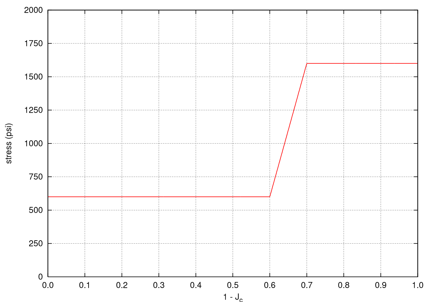
Fig. 5.10 An example of an input crush curve for an aluminum honeycomb.
Above some value of compaction (\(1-J_c=V_{min}\)), the material will be fully compacted and behave as an elastic, perfectly plastic material. The fully compacted response is given by the Young’s modulus, \(E\), Poisson’s ratio, \(\nu\), and the yield stress, \(\sigma_{y}\). Details of this response may be found in previous sections on the various elastic-plastic models (e.g. Section 5.2.5).
In the above command blocks:
The
EX,EY,EZ,GXY,GYZ, andGZXcommand lines define, respectively, the initial, pre-crush directional moduli \(E_{xx}\), \(E_{yy}\), \(E_{zz}\), \(G_{xy}\), \(G_{yz}\), and \(G_{zx}\) from (5.83).CRUSHXX,YY,ZZ,XY,YZ, andZXinputs require the name of a function defined via aFUNCTIONcommand line in the SIERRA scope. These functions describe the directional crush characteristics of the material and give the current stress value (in a direction) as a function of the current compaction (\(1-J_c\)).The command
VMINdefines the minimum relative volume of the material that is achieved when the material is completely crushed. This parameter may also be considered as the maximum compaction.The elastic constant commands refer to the post lock-up, fully compacted isotropic response of the material. See Section 5.1.5 for more information on elastic constants input.
YIELD STRESSrefers to the plateau stress of the material after lock-up when the response is perfectly plastic.
Output variables available for this model are listed in Table 5.25. For information about the orthotropic crush model, consult [[42]].
Name |
Description |
|---|---|
|
current (unrecoverable) compaction/relative volume |
5.2.29. Orthotropic Rate Model
BEGIN PARAMETERS FOR MODEL ORTHOTROPIC_RATE
  #
  # Elastic constants
  #
  YOUNGS MODULUS = <real>
  POISSONS RATIO = <real>
  SHEAR MODULUS  = <real>
  BULK MODULUS   = <real>
  LAMBDA         = <real>
  TWO MU         = <real>
  #
  YIELD STRESS = <real>
  #
  MODULUS TTTT = <real>
  MODULUS TTLL = <real>
  MODULUS TTWW = <real>
  MODULUS LLLL = <real>
  MODULUS LLWW = <real>
  MODULUS WWWW = <real>
  MODULUS TLTL = <real>
  MODULUS LWLW = <real>
  MODULUS WTWT = <real>
  #
  TX = <real>
  TY = <real>
  TZ = <real>
  LX = <real>
  LY = <real>
  LZ = <real>
  #
  MODULUS FUNCTION = <string>
  RATE FUNCTION    = <string>
  #
  T FUNCTION  = <string>
  L FUNCTION  = <string>
  W FUNCTION  = <string>
  TL FUNCTION = <string>
  LW FUNCTION = <string>
  WT FUNCTION = <string>
END [PARAMETERS FOR MODEL ORTHOTROPIC_RATE]
The orthotropic rate model extends the functionality of the orthotropic crush constitutive model described in Section 5.2.28. The orthotropic rate model has been developed to describe the behavior of an aluminum honeycomb subjected to large deformation. The orthotropic rate model, like the original orthotropic crush model, has six independent yield functions that evolve with volume strain. Unlike the orthotropic crush model, the orthotropic rate model has yield functions that also depend on strain rate. The orthotropic rate model also uses an orthotropic elasticity tensor with nine elastic moduli in place of the orthotropic elasticity tensor with six elastic moduli used in the orthotropic crush model.
A honeycomb orientation capability is included with the orthotropic rate model, allowing users to prescribe initial honeycomb orientations that are not aligned with the original global coordinate system. The three material directions are defined as follows: The T-direction is usually associated with the generator axis for the honeycomb, the L-direction is in the ribbon plane (defined by flat sheets used in reinforced honeycomb) orthogonal to the generator axis, and the W-direction is orthogonal to the ribbon plane.
In the above command blocks:
For the
ORTHOTROPIC_RATEmodel, onlyYOUNGS MODULUSneeds to be defined; this is the Young’s modulus in the fully compacted state. If two other elastic constants are provided, they will be used to define the fully compacted Young’s modulus. See Section 5.1.5 for more information on elastic constants input.The
YIELD STRESScommand line defines the yield stress of the fully compacted honeycomb.The nine elastic moduli for the orthotropic, uncompacted honeycomb are defined with respect to each material direction using the
MODULUS TTTT,MODULUS TTLL,MODULUS TTWW,MODULUS LLLL,MODULUS LLWW,MODULUS WWWW,MODULUS TLTL,MODULUS LWLW, andMODULUS WTWTcommand lines.The components of vectors defining the T- and L-directions of the honeycomb are specified using the
TX,TY, andTZ, andLX,LY, andLZcommand lines, respectively. The vector component valuestx,ty, andtzdefine the orientation of the honeycomb’s T-direction (generator axis), whilelx,ly, andlzdefine the orientation of the L-direction. The vectors T and L are defined in the global coordinate system and must be orthogonal.The function describing the variation in moduli with compaction is given by the
MODULUS FUNCTIONcommand line. The moduli vary continuously from their initial orthotropic values to isotropic values when full compaction is obtained.The function describing the change in strength with strain rate is given by the
RATE FUNCTIONcommand line. Note that all strengths are scaled with the multiplier obtained from this function.The function describing the T-normal strength of the honeycomb as a function of compressive volumetric strain is given by the
T FUNCTIONcommand line.The function describing the L-normal strength of the honeycomb as a function of compressive volumetric strain is given by the
L FUNCTIONcommand line.The function describing the W-normal strength of the honeycomb as a function of compressive volumetric strain is given by the
W FUNCTIONcommand line.The function describing the TL-normal strength of the honeycomb as a function of compressive volumetric strain is given by the
TL FUNCTIONcommand line.The function describing the LW-normal strength of the honeycomb as a function of compressive volumetric strain is given by the
LW FUNCTIONcommand line.The function describing the WT-normal strength of the honeycomb as a function of compressive volumetric strain is given by the
WT FUNCTIONcommand line.
Note that several of the command lines in this command block reference functions. These functions must be defined in the SIERRA scope.
Output variables for this model are listed in Table 5.26.
Index |
Name |
Variable Description |
|---|---|---|
1 |
|
minimum volume ratio, crush is unrecoverable \(\left(\hat{\varepsilon}_{V}\right)\) \ |
Warning
Strongly rate-dependent models may fare poorly in implicit quasistatic solution. In implicit analyses the rate term used to evaluate the current load step is the rate seen by the model in the previous load step. This may cause the solution to oscillate between high- and low-rate equilibrium states from step to step.
5.2.30. Plane Stress Rate Plasticity
BEGIN PARAMETERS FOR MODEL PLANE_STRESS_RATE_PLASTICITY
   #
   # Elastic constants
   #
   YOUNGS MODULUS = <real>
   POISSONS RATIO = <real>
   SHEAR MODULUS  = <real>
   BULK MODULUS   = <real>
   LAMBDA         = <real>
   TWO MU         = <real>
   #
   # Optional parameters related to inelastic correction criteria
   #
   TOLERANCE          = <real> tolerance (1.0e-10)
   MAX_INEL_CORR_ITER = <int> maximum_correction_iterations (100)
   MAX_LS_CORR_ITER   = <int> maximum_line_search_cutbacks  (20)
   #
   USER RATE DEPENDENCE = 0|1(0)
   YIELD STRESS         = <real>
   #
   FORMULATION          = <int> formulation (1)
   #
   # Input Options for USER RATE DEPENDENCE = 0
   #
   # linear hardening
   HARDENING MODULUS = <real> hardening_modulus
   # power law hardening
   HARDENING CONSTANT = <real> hardening_constant
   HARDENING EXPONENT = <real> hardening_exponent (0.5)
   # multilinear hardening
   HARDENING FUNCTION = <string>
   #
   # Rate dependence
   #
   # Johnson-Cook rate dependence
   RATE CONSTANT = <real>
   # multilinear rate dependence
   RATE FUNCTION = <string> rate_function_name
   #
   # Input Options for USER RATE DEPENDENCE = 1
   #
   # rate-dependent yield
   YIELD STRAIN RATES = <real_list> yield_strain_rates
   YIELD CURVES       = <string_list> yield_function_names
   # rate-dependent damage
   FRACTURE STRAIN RATES = <real_list> fracture_strain_rates
   FRACTURE CURVES       = <string_list> fracture_function_names
   DECAY COEFFICIENT     = <real> (1.0)
   #
   # Thermal softening commands (Johnson-Cook)
   INITIAL TEMPERATURE   = <real>
   MELT TEMPERATURE      = <real>
   REFERENCE TEMPERATURE = <real>
   THERMAL EXPONENT      = <real>
   #
END [PARAMETERS FOR MODEL PLANE_STRESS_RATE_PLASTICITY]
The plane stress rate plasticity model is the plane stress formulation of a \(J_2\) plasticity model given by Simo and Taylor [[43]] (and described again in Simo and Hughes [[5]]) extended to include rate-dependent hardening and a failure model for use with shell elements.
Like other plasticity models, the components of the objective stress rate, \(\stackrel{\circ}{\sigma}_{ij}\), are written as,
where \(\mathbb{C}_{ijkl}\) are the components of the fourth-order, isotropic elasticity tensor and \(D_{ij}^{\text{e}}\) are the components of the elastic part of the total rate of deformation tensor. An additive split of the total rate of deformation tensor into elastic and plastic contributions is assumed such that,
The plane stress formulation recasts the three-dimensional problem into a constrained subspace with plane stress conditions acting as the constraints. To do this, the plane stress rate plasticity model follows the approach of Simo and Taylor [[43]] to enforce \(\sigma_{13}=\sigma_{23}=\sigma_{33}=0\) and related conditions.
For the plasticity portion of the model, the formulation of Simo and Taylor [[43]] is usedfootnote{In the work of Simo and Taylor [[43]] (and later Simo and Hughes [[5]]) hardening is assumed to be rate and temperature independent. Here, such terms are included but do not materially change the formulation. Similarly, the earlier works also introduce kinematic hardening which is not used in the current model.} in which a traditional three-dimensional \(J_2\) plasticity model is recast in reduced subspace. To do this, it is recalled that in three-dimensions the von Mises effective stress, \(\phi\), is written,
with \(s_{ij}=\sigma_{ij}-(1/3)\sigma_{kk}\delta_{ij}\) the deviatoric stress. To write an equivalent expression in the reduced subspace, the vector, \(\underline{\sigma}\), and matrix, \(\underline{\underline{\bar{P}}}\), are introduced asfootnote{Note, here the \(\underline{x}\) and \(\underline{\underline{X}}\) notations are introduced for vector and matrix objects, respectively, to clearly distinguish that these variables are not tensors. This results from operating in the constrained stress subspace and means that these terms do not have properties of a tensor and act on each other as traditional matrices and vectors.},
such that,
In the reduced plane-stress subspace, an alternative effective stress, \(\bar{\phi}\), is given as,
where
in which \(\underline{\underline{P}}\) and \(\underline{\underline{\bar{P}}}\) differ by a two in the shear term to reflect Voigt corrections.
A yield function, \(f\), is introduced as,
with,
where \(\bar{\varepsilon}^p\) and \(\dot{\bar{\varepsilon}}^p\) are the equivalent plastic strain (isotropic hardening variable) and its rate, respectively. Various hardening options may be used with this model. In general, the current flow stress is written as,
in which \(\sigma_y\) is the original yield stress, \(K\) is the isotropic hardening function that may take linear, power-law, or multilinear form, \(\hat{\sigma}\) the rate multiplier whose specification will be defined later, and the right-most term is the Johnson-Cook temperature dependence term that may be optionally used to give temperature dependence of the flow-stress.
To complete the theoretical formulation, the flow rules are specified as,
where \(\lambda\) is the consistency multiplier enforcing \(f=0\) during plastic deformation and \(d\underline{\varepsilon}^p\) is the plastic strain increment in the constrained subspace. It is emphasized here that the yield surface described in (5.85) is not homogeneous of degree one like in other three-dimensional formulations presented in this manual. As such, the consistency multiplier and equivalent plastic strain increment are not equivalent. As an example of this, by consideration of the preceding relations, it is apparent that \(\lambda\) has units of one over stress.
The specification of the rate dependence, \(\hat{\sigma}\), is important as it enables the consideration of two different model responses. These behaviors are controlled via the USER RATE DEPENDENCE command. If this input parameter is zero, then either an analytical or user-defined rate-dependence may be given. Importantly, in this case failure is not modeled. For the analytical case, the Johnson-Cook [[8], [9]] rate-multiplier is used such that,
with \(C\) being the rate dependence multiplier and \(\dot{\bar{\varepsilon}}_0\) is a reference rate. Note, while other models allow user specification of the reference rate, the plane stress rate plasticity model uses the value set in the original work of Johnson-Cook [[8]] such that \(\dot{\bar{\varepsilon}}_0=1 \text{s}^{-1}\). Alternatively, a user function may be specified for the rate multiplier, \(\hat{\sigma}\).
If USER RATE DEPENDENCE is set to one, both rate dependence and failure may be modeled. With respect to the rate dependence, (5.86) is rewritten,
in which both isotropic hardening and rate dependence are described via definition of \(\tilde{\sigma}\). In this case, \(\tilde{\sigma}\) can*not* be specified through analytical expressions and must instead be given as a series of isotropic hardening curves; each at a different strain rate. For rates not explicitly given, interpolation is performed between relevant curves. Note, no extrapolation is performed with respect to the rates. If a rate is determined outside any specified curves, the hardening is calculated with respect to the bounding curve.
For failure, a failure parameter, \(\alpha\), is calculated as
in which the summation is used to imply the discrete calculation of the damage variable over a series of loadsteps and \(\varepsilon_f\) is the rate and triaxiality, \(\eta\), dependent failure strain. The failure strain, \(\varepsilon_f\), is specified in a fashion similar to \(\tilde{\sigma}\). Specifically, a series of triaxiality dependent functions are defined each at a given strain rate. Interpolation is used at rates between those specified. Extrapolation outside the defined bounds is not done and the extremum curves are instead used.
The onset of damage is assumed to occur when \(\alpha = 1\) and the current failure strain is taken to be the critical one such that \(\varepsilon_f^{cr}=\varepsilon_f\left(t=t_{cr}\right)\) with \(t_{cr}\) being the time at which \(\alpha=1\). Subsequent damage calculation is performed via,
After the critical failure parameter has been reached, an exponential decay relation is used to decrease the strength of the material. In this fashion, a decay relation of the form,
is used in which \(C_1\) is the decay coefficient.
For more information about the plane stress rate plasticity model, consult [[43], [5]].
In the command blocks that define the Plane Stress Rate Plasticity model:
See Section 5.1.5 for more information on elastic constants input.
TOLERANCEspecifies the numerical value used for assessing convergence of the plastic correction routine.Optionally, the user can specify the maximum number of inelastic correction iterations for the plasticity inelastic correction routines. By default this value is 100.
Optionally, the user can specify the maximum number of line search cutbacks in the plasticity correction routine. By default this value is 20 and only impacts the formulation not equal to 0 (plastic strain rate) case.
The reference nominal yield stress, \(\bar{\sigma}\), is defined with the
YIELD STRESScommand line.The formulation parameter defines whether the total strain rate (formulation = 0) or equivalent plastic strain rate (anything else) is used for calculating rate dependence.
INITIAL TEMPERATUREdefines the initial temperature at \(t=0\).MELT TEMPERATUREdefines \(T_{melt}\) in (5.86).REFERENCE TEMPERATUREdefines \(T_{ref}\) in (5.86).THERMAL EXPONENTdefines \(M\) in (5.86).The
USER RATE DEPENDENCEis used to control the way hardening may be specified and whether or not failure is calculated.For
USER RATE DEPENDENCE = 0, plastic hardening may be specified as linear, power-law, OR multilinear. Failure cannot be used withUSER RATE DEPENDENCE = 0:For linear hardening, a non-zero
HARDENING MODULUSshould be specified. Do not give if using power-law or multilinear hardening.For power-law hardening, the
HARDENING CONSTANTshould be specified. Optionally, theHARDENING EXPONENTparameter should be specified if the default value (0.5) is not to be used. Do not give for linear or multilinear hardening.For multilinear hardening, a function name should be given for
HARDENING FUNCTIONcommand. Do not specify for linear or power-law hardening.For Johnson-Cook rate-dependence, a rate constant must be specified via the
RATE CONSTANTcommand. Do not use if using functionally specified rate-dependence.For functionally defined rate-dependence, a function name should be given via the
RATE FUNCTIONcommand. Do not specify if using Johnson-Cook type rate dependence.
For
USER RATE DEPENDENCE = 1, plastic hardening is specified through a series of user functions. Failure can be modeled withUSER RATE DEPENDENCE = 1:Rate-dependent plastic hardening is specified jointly via the
YIELD STRAIN RATESandYIELD CURVEScommands.YIELD STRAIN RATESis a list of strain rates corresponding one-to-one to functions specified in theYIELD CURVESlist of strings giving user-defined function names. EachYIELD CURVESfunction should give the plastic isotropic plastic hardening curve at the corresponding rate given inYIELD STRAIN RATES.Failure strains used in calculating damage are specified via the
FRACTURE STRAIN RATESandFRACTURE CURVEScommands. Similarly to the plastic hardening, a list of strain rates should be given with theFRACTURE STRAIN RATESinput. Each rate should correspond one-to-one with a user function listed viaFRACTURE CURVES. These functions are specified as a function of triaxiality and should give the failure strain at the specified rate.The decay coefficient, \(C_1\), that controls the exponential decay of the yield stress related to failure should be specified via the
DECAY COEFFICIENTcommand.
Output variables available for this model are listed in Table 5.27.
Name |
Description |
|---|---|
|
equivalent plastic strain, \(\bar{\varepsilon}^{p}\) |
|
equivalent plastic strain rate, \(\dot{\bar{\varepsilon}}^{p}\) |
|
effective stress, \(\phi\) |
Warning
Strongly rate-dependent models may fare poorly in implicit quasistatic solution. In implicit analyses the rate term used to evaluate the current load step is the rate seen by the model in the previous load step. This may cause the solution to oscillate between high- and low-rate equilibrium states from step to step.
5.2.31. Incompressible Solid Model
BEGIN PARAMETERS FOR MODEL INCOMPRESSIBLE_SOLID
  #
  # Elastic constants
  #
  YOUNGS MODULUS = <real>
  POISSONS RATIO = <real>
  SHEAR MODULUS  = <real>
  BULK MODULUS   = <real>
  LAMBDA         = <real>
  TWO MU         = <real>
  #
  #
  #
  K SCALING = <real>k_scaling
  2G SCALING = <real>2g_scaling
  TARGET E = <real>target_e
  MAX POISSONS RATIO = <real>max_poissons_ratio
  REFERENCE STRAIN = <real>reference_strain
  SCALING FUNCTION = <string>scaling_function_name
END [PARAMETERS FOR MODEL INCOMPRESSIBLE_SOLID]
The incompressible solid model is a variation of the elastic model and can be used in both Presto and Adagio. In Adagio, the incompressible solid model is used with the control-stiffness option in the multilevel solver. The control-stiffness option is implemented via the CONTROL STIFFNESS command block and is discussed in Section 4. The model is used to model nearly incompressible materials where Poisson’s ratio, \(\nu\), \(\approx 0.5\). In the course of solving a series of model problems in Adagio, the material response from this model incorporates scaling the bulk and/or shear behaviors to yield a material response that is more amenable to solution using Adagio’s conjugate gradient solver. The final material behavior that is calculated corresponds to the actual moduli that are specified. When this model is used in Presto, the material scalings are ignored, and the model behaves like a linear elastic model.
In the above command blocks, the following definitions are applicable. Usage requirements are identified both in this list of definitions and in the discussion that follows the list.
See Section 5.1.5 for more information on elastic constants input.
The following material-scaling command lines are used only in Adagio and are optional as described below: - The nominal bulk scaling is defined with the
K SCALINGcommand line. - The nominal shear scaling is defined with the2G SCALINGcommand line. - The target Young’s modulus is defined with theTARGET Ecommand line. - The maximum Poisson’s ratio is defined with theMAX POISSONS RATIOcommand line. - The reference strain is defined with theREFERENCE STRAINcommand line. - TheSCALING FUNCTIONcommand line references the name of a function defined in aFUNCTIONcommand line in the SIERRA scope that describes the time dependent scaling to be applied.
As noted previously, only two of the elastic constants are required to define the unscaled material response. This requirement applies to use of the incompressible solid model in Presto and in Adagio. Further, all the material-scaling command lines are only used in Adagio.
Several options exist for defining the bulk and/or shear scalings that can be used with the multilevel solver in Adagio.
Option 1: You can provide the scalings directly by including both of the
K SCALINGand2G SCALINGcommand lines or either of them. When both command lines are input, the user-specified values for their parameters will be used. If only theK SCALINGcommand line is input, the bulk scaling is as specified in thek_scalingparameter, and the value of the shear scaling parameter,2g_scaling, is set to 1.0. On the other hand, if only the2G SCALINGcommand line is input, then the shear scaling is as specified in the2g_scalingparameter, but the value of the bulk-scaling parameter,k_scaling, is not set to 1.0. Instead, the bulk scaling is determined by computing a scaled bulk modulus from the scaled shear modulus and a (scaled) Poisson’s ratio of 0.3. Then, the bulk scaling is determined as the ratio of the scaled bulk modulus to the actual bulk modulus.Option 2: You can specify either or both of the
TARGET EandMAX POISSONS RATIOcommand lines to define the scalings. If only theTARGET Ecommand line is included, the bulk and shear scalings are computed by first finding scaled moduli using the value of thetarget_eparameter along with a (scaled) Poisson’s ratio of 0.3. The bulk and shear scalings are then determined as the ratio of the appropriate scaled to unscaled modulus. If only theMAX POISSONS RATIOcommand line is included, the shear scaling is set to 1.0, and the bulk scaling is computed by first calculating a scaled bulk modulus from the actual shear modulus and the value of themax_poissons_ratioparameter. The bulk scaling is then calculated as the ratio of the scaled bulk modulus to the actual bulk modulus. If both theTARGET EandMAX POISSONS RATIOcommand lines are included, the bulk scaling (and shear scaling) is determined from the ratio of the bulk scaled modulus (and shear scaled modulus) computed using the values of thetarget_eandmax_poissons_ratioparameters to the unscaled bulk (and shear) modulus.Option 3: You can choose not to include any of the
K SCALING,2G SCALING,TARGET E, andMAX POISSONS RATIOcommand lines. In such case, the shear scaling is set to 1.0, and the bulk scaling is computed as the ratio of the scaled bulk modulus coming from the real shear modulus and a (scaled) Poisson’s ratio of 0.3 to the actual bulk modulus.
The function referenced by the value of the parameter scaling_function_name in the SCALING FUNCTION command line can be used to modify the bulk and shear scalings in solution time. The actual scalings used are computed by taking the scalings specified by the parameter values in the K SCALING, 2G SCALING, TARGET E, and MAX POISSONS RATIO command lines and multiplying them by the function value at the specified solution time. If the SCALING FUNCTION command line is not included, the bulk and shear scalings are fixed in time.
The REFERENCE STRAIN command line supplies a value for the reference strain that is used to create a normalized material constraint violation based on strains. Specifying a reference strain implies the use of strains for measuring the material constraint violation (or part of the control-stiffness error in Adagio). Otherwise, the material constraint violation is determined by using the change in the scaled stress response over the current model problem.
5.2.32. Universal Polymer Model
The UPM model is commonly used in one of two ways. The most general use case is portrayed in full in the following syntax in which the user specifies both Prony series explicitly. That is, the user specifies all Prony relaxation times (\({\tau}\)) and weights for both the thermal/volumetric (\({f_v}\)) and shear (\({f_s}\)) relaxation functions. Note that in the UPM model, only a single set of Prony relaxation times can be specified and acts as the basis for both relaxation spectra. In other words, a single set of relaxation times is specified, and both functions use their own (distinct) weights.
Default parameters are not set. Any system of units can be used with the model. There are no internalunits assumptions.
BEGIN PARAMETERS FOR MODEL UNIVERSAL_POLYMER
  #
  # Elastic constants: These Should be Set to the Glassy Moduli
  #                    for robustness considerations
  #
  SHEAR MODULUS  = <real>
  BULK MODULUS   = <real>
  #
  ## Reference Temperature and Material CLOCK Parameters
  #
  REFERENCE TEMPERATURE   = <real> # Temperature
  STRESS FREE TEMPERATURE = <real>  # Temperature
  #
  WLF C1   = <real>
  WLF C2   = <real> # Temperature
  CLOCK C3 = <real> # Temperature
  CLOCK C4 = <real> # Temperature
  #
  ## Glassy and Rubbery Moduli
  #  and CTE Definitions at the Reference Temperature
  #
  BULK GLASSY 0    = <real> # Units of Pressure
  BULK RUBBERY 0   = <real> # Units of Pressure
  SHEAR GLASSY 0   = <real> # Units of Pressure
  SHEAR RUBBERY 0  = <real> # Units of Pressure
  VOLCTE glassy 0  = <real> # Units of Inverse Temperature
  VOLCTE rubbery 0 = <real> # Units of Inverse Temperature
  #
  FILLER VOL FRACTION = <real>
  #
  ## Relaxation Time Spectra Definitions
  #
  WWBETA 1 = <real>
  WWTAU 1  = <real> # Units of time
  WWBETA 2 = <real>
  WWTAU 2  = <real> # Units of time
  #
  SPECTRUM START TIME = <real>  # Units of time
  SPECTRUM END TIME   = <real>  # Units of time
  LOG TIME INCREMENT  = <real>  # Units of time
  #
  ## Direct Prony Spectra Inputs
  #
  RELAX TIME 1 = <real>  # Unit of time
  RELAX TIME 2 = <real>
  .
  RELAX TIME 30 = <real>
  #
  ## Thermal/Volumetric Relaxation Spectrum Prony Weights
  #
  F1 1 = <real>
  F1 2 = <real>
  .
  F1 30 = <real>
  #
  ## Shear Relaxation Spectrum Prony Weights
  #
  F2 1 = <real>
  F2 2 = <real>
  .
  F2 30 = <real>
 END [PARAMETERS FOR MODEL UNIVERSAL_POLYMER]
Not all Prony spectra/weight parameter pairs (1-30) need to be specified. Only those specified will be used, and the ones not specified will be set to zero. Prony weights for each relaxation function should sum to 1.0, or the model will rescale the weights so that they do sum to one. This rescaling will change the underlying relaxation response.
When the model is used with both relaxation functions being specified directly, then the parameters: SPECTRUM START TIME, SPECTRUM END TIME, LOG TIME INCREMENT, WW TAU (1,2), and WW BETA (1,2) must be specified as 0 to avoid errors during the model property check. Note (1) is associated with the thermal/volumetric function, and (2) is associated with the shear relaxation function.
Another common usage of the UPM model is to specify the Williams-Watts (KWW) stretched exponential \(\tau, \beta\) parameters for either or both relaxation functions (1 and/or 2) corresponding to the function \(f=\exp(-(t/\tau)^\beta)\). That is, a set of Prony weights, \(w_i\) corresponding to a specific set of Prony times, \(\tau_i\), will be found during the model property check routine. If the other relaxation function is directly specified as above, then the Prony times from the directly specified relaxation spectrum are used. In this case, the Prony weights for the relaxation function being fit to the KWW function are found through a Least-Squared Error minimization routine built into the UPM model over a discretely sampled set of times between the minimum and maximum Prony times.
When neither Prony spectrum is directly specified (both will be fit to KWW functions), then the Prony times (for both relaxation functions) are determined from an evenly logarithmically spaced set of Prony times beginning with the SPECTRUM START TIME and ending with the SPECTRUM END TIME and spaced with the (base 10) LOG TIME INCREMENT. For each relaxation function that is fit with the UPM model to a KWW function, the WW TAU (1,2) and WW BETA (1,2) parameters must be specified. However, if the user specifies both a KWW form and the same Prony series directly, the model will error out during the property check.
There are many useful optional parameters for the UPM model that generally allow for: temperature dependence of moduli, coefficients of thermal expansion, deformation dependence of moduli, and/or alternative material clock parameter specifications. These parameters may optionally be added to the material input block, but are defaulted to 0.0:
### OPTIONAL parameters for the universal_polymer model
 CLOCK C1         = <real> # CLOCK Coef. 1 instead of "WLF C1"
 CLOCK C2         = <real> # CLOCK Coef. 1 instead of "WLF C2"
 BULK GLASSY 1    = <real> # Pressure per Temperature
 BULK RUBBERY 1   = <real> # Pressure per Temperature
 SHEAR GLASSY 1   = <real> # Pressure per Temperature
 SHEAR RUBBERY 1  = <real> # Pressure per Temperature
 VOLCTE GLASSY 1  = <real> # Inverse Temperature Squared
 VOLCTE RUBBERY 1 = <real> # Inverse Temp. Squared
Finally, we note that the UPM model may be reduced to a finite deformation, linear thermoviscoelastic model by choosing \(C_3 = 0\) and \(C_4 = 0\). Under these conditions the material clock is only temperature (history) dependent but involves no deformation dependence. Moreover, if one wants to fix the laboratory and material time scales to be the same, then one should set WLF \(C_1\) = 0.
The Universal Polymer Model (UPM) is a phenomenological, non-linear viscoelastic (NLVE) model that is, in the literature, named the Simplified Potential Energy Clock (SPEC) [[44]]. The UPM model is considerably simpler than the parent model, the Potential Energy Clock (PEC) model, labeled the NLVE polymer model in SIERRA, which itself is not phenomenological but requires extensive data and experience to calibrate [[45]].
The UPM model is suitable for modeling the finite deformation, thermal-mechanical behavior of glassy materials, both organic and inorganic. Successful usage of the model is widespread. Some examples include the modeling of amorphous, thermosetting polymers across and through the glass transition such as epoxies [[46]]. It is also suitable for modeling thermoplastics from within the melt state and down into the glass transition from polystyrene to polycarbonate. Finally, it has been used to represent inorganic glasses for glass-to-metal seals. The UPM model was developed for production analyses of encapsulated components. It predicts a full range of behavior including yielding, stress relaxation, volume relaxation, and physical aging.
The key physical principal behind the UPM model is that there exists a material time scale (material clock) separate from the laboratory time scale. If the material time scale is fast, such as in the rubbery state of a polymer, then the UPM model responds instantly to changes in temperature and strain such that the user would observe rate-independent behavior. However, if the material clock is slow relative to the laboratory time scale, viscoelastic memory builds with any process, which causes acute history and thermodynamic path dependent behavior.
The model response is derived from a Helmholtz Free Energy density and takes as an input the unrotated rate of deformation, \(d_{ij}\), the temperature at the start and end of the time step \(\theta_{n}\) and \(\theta_{n+1}\), and the time step, \(\Delta\,t\). From these inputs, the hereditary integrals within the model are updated, and the unrotated Cauchy stress tensor is returned.
For the UPM model, the strain measure is approximated from the integrated unrotated rate of deformation tensor, which we label \(\epsilon_{ij}\),
Here, \(F_{ij}\), \(R_{ij}\), \(U_{ij}\), \(L_{ij}\), and \(D_{ij}\) are the deformation gradient, rotation, material stretch, velocity gradient, and rate of deformation tensors standard in Lagrangian continuum mechanics.
The UPM model allows the user to initiate an analysis from a stress-free temperature, \(\theta_{\rm sf}\), that is different from the reference temperature, \(\theta_{\rm ref}\), at which all material properties are defined. Here we briefly summarize the constitutive equations. The model is derived from a Helmholtz Free Energy, but we begin directly with the (unrotated) Cauchy Stress and refer the reader to reference [[44]] for more detail:
The first three lines of terms in (5.87) represent the time-dependent and dissipative (non-equilibrium) response of the model to volumetric, thermal, and shear deformation histories. Accordingly, \(K\), \(\delta\), and \(G\) represent a bulk modulus, volumetric thermal expansion coefficient, and shear modulus while subscripts \(_G\) or \(_\infty\) denote a glassy or rubbery, respectively, properties. The last collection of terms in (5.87) furnish the time-independent rubbery (equilibrium) response. The variables in equation (5.87) are:
The first three terms in (5.87) represent the material’s viscoelastic response to changes in volume strain, temperature, and shear deformation. Two relaxation functions are used to characterize the thermal/volumetric (\(f_v\)) and shear (\(f_v\)) relaxation responses. The model assumes the thermal and volumetric relaxation responses are identical. Otherwise, \(f_v\) and \(f_s\) are typically quite different and are expressed as a Prony series footnote{Note: to distinguish between indices used with conventional summation convention and those related to Prony series terms, all Prony series summations shall be explicitly written with the relevant index given parenthetically in a superscript.}:
These relaxation functions describe the material’s response to a suddenly applied volumetric/thermal or shear perturbation at the reference temperature where, under certain conditions, the material and laboratory time scales are equivalent. In (5.87), the viscous terms (non-rubbery) involve hereditary integrals over the difference in material time from \(s=0\) to \(s=t\), which is the current laboratory time.
An increment in material time, \(dt'\), and the laboratory time, \(dt\), are related through the (highly) history dependent shift factor, \(a\), such that the difference in material time, \(t' - s'\), is related to the corresponding difference in laboratory time, \(t - s\) through:
If the material time scale is very slow compared to the laboratory time, then \(a>>1\), which is often the case inside and below the glass transition for typically glassy materials.
The shift factor is instantaneously defined through:
The key physics in the model comes form (5.90). Temperature rise (generally) causes \(N\) to increase, and hence the material shift factor shrinks (the material time scale speeds up). Shrinking the volume generally causes the shift factor to increase as if the temperature had been decreased. Mechanistically, this feature is the manifestation of the trade-off between between mobility and free volume available to polymer chains. Finally, shear deformation can greatly speed up the material clock through the last term. This phenomenon is a direct manifestation of “deformation induced mobility”, a key mechanism for glassy materials.
Since the shift factor involves hereditary integrals, even at a constant temperature and state of deformation, the material clock will change over time. Under stress-free conditions, the material will creep and densify if the model is out of equilibrium (when any viscous term is non-zero). These phenomena are the model’s manifestations of physical aging, time-dependent material change without a change in composition or microstructure. \(C_1\), \(C_2\), \(C_3\), and \(C_4\) are all material constants. We note that the double relaxation function appearing in the last term takes on a slightly different form from \(f_s\):
It is desirable to relate a special case of the model to the Williams-Landel-Ferry (WLF) form because of how time-temperature superposition fitting is typically performed. Specifically, one can show that the clock parameters, \(C_1\) and \(C_2\), relate to the WLF parameters, \(\hat{C}_1\) and \(\hat{C}_2\), through the following relationships: \(\hat{C}_1 = C_1\) and \(\hat{C}_2 = C_2 /\left(1 + C_3 \delta_{\infty}^{\rm ref} \right)\).
For more information about the universal polymer model, consult [[44]].
Output variables available for this model are listed in Table 5.28. The user should always output the shift factor \(aend\) or log:math:_{10}a as this variable is critical for interpreting the material behavior.
Name |
Description |
|---|---|
|
The shift factor relating increments of material to laboratory time, \(a\, dt^* = dt_{\rm lab}\) |
|
\({\rm log_{10}}\) of the shift factor, \({\rm log_{10}}a\) |
|
xx component of the integrated unrotated rate of deformation, \(\epsilon_{xx}\) |
|
yy component of the integrated unrotated rate of deformation, \(\epsilon_{yy}\) |
|
zz component of the integrated unrotated rate of deformation, \(\epsilon_{zz}\) |
|
xy component of the integrated unrotated rate of deformation, \(\epsilon_{xy}\) |
|
yz component of the integrated unrotated rate of deformation, \(\epsilon_{yz}\) |
|
zx component of the integrated unrotated rate of deformation, \(\epsilon_{zx}\) |
|
second (non-Cayley Hamilton) invariant of \(\epsilon\) providing shear deformation, \(I_2\) |
|
volumetric hereditary integrals 1-30 |
|
thermal hereditary integrals 1-30 |
|
xx component shear hereditary integrals 1-30 |
|
yy component shear hereditary integrals 1-30 |
|
zz component shear hereditary integrals 1-30 |
|
xy component shear hereditary integrals 1-30 |
|
yz component shear hereditary integrals 1-30 |
|
zx component shear hereditary integrals 1-30 |
5.2.33. Mooney-Rivlin Model
BEGIN PARAMETERS FOR MODEL MOONEY_RIVLIN
  #
  # Elastic constants, One of these elastic constants must be input.
  # The shear modulus is computed from C10 and C01.
  #
  YOUNGS MODULUS = <real>
  POISSONS RATIO = <real>
  BULK MODULUS   = <real>
  LAMBDA         = <real>
  #
  #
  C10 = <real>c10
  C01 = <real>c01
  C10 FUNCTION = <string>c10_function_name
  C01 FUNCTION = <string>c01_function_name
  BULK FUNCTION = <string>bulk_function_name
  THERMAL EXPANSION FUNCTION = <string>eth_function_name
  TARGET E = <real>target_e
  TARGET E FUNCTION = <string>etar_function_name
  MAX POISSONS RATIO = <real>max_poissons_ratio(0.5)
  REFERENCE STRAIN = <real>reference_strain
END [PARAMETERS FOR MODEL MOONEY_RIVLIN]
Mooney-Rivlin is a hyperelastic material model that is used to describe rubber. The Mooney-Rivlin model incorporates temperature-dependent material moduli and can be used in both Presto and Adagio. When the model is used in Adagio, it can be used with or without the control-stiffness option in Adagio’s multilevel solver. The control-stiffness option is implemented via the CONTROL STIFFNESS command block and is discussed in Section 4. The model is used to simulate nearly incompressible materials where Poisson’s ratio, \(\nu\), \(\approx 0.5\). In the course of solving a series of model problems in Adagio, the material response from this model incorporates scaling the bulk and/or shear behaviors to yield a material response that is more amenable to solution using Adagio’s conjugate gradient solver. The final material behavior that is calculated corresponds to the actual moduli that are specified. When this model is used in Presto, the material scalings are ignored.
In the above command blocks the following command lines are required:
The material constants C10 and C01 determine the shear behavior as defined by
(5.92)\[\texttt{shear\_modulus} = 2 \left(C_{10} + C_{01}\right).\]Thus the
C10andC01command lines must be included in this model and the shear modulus elastic constant is not an available input.Since
C10andC01define the shear behavior, one additional elastic constant, other than the shear modulus is required to define the unscaled bulk behavior. See Section 5.1.5 for more information on elastic constants input.
Other command line options include:
The
C10 FUNCTIONcommand line references the name of a function defined in aFUNCTIONcommand line in the SIERRA scope that describes the temperature dependence of the C10 material parameter. This command line is optional. If it is not present, there is no temperature dependence in the C10 parameter. See the usage discussion below.The
C01 FUNCTIONcommand line references the name of a function defined in aFUNCTIONcommand line in the SIERRA scope that describes the temperature dependence of the C01 material parameter. This command line is optional. If it is not present, there is no temperature dependence in the C01 parameter. See the usage discussion below.The
BULK FUNCTIONcommand line references the name of a function defined in aFUNCTIONcommand line in the SIERRA scope that describes the temperature dependence of the bulk modulus. This command line is optional. If it is not present, there is no temperature dependence in the bulk modulus. See the usage discussion below.The
THERMAL EXPANSION FUNCTIONcommand line references the name of a function defined in aFUNCTIONcommand line in the SIERRA scope that describes the linear thermal expansion as function of temperature. This command line is optional. If it is not present, there is no thermal expansion. See the usage discussion below.The following material-scaling command lines are used only in Adagio:
The target Young’s modulus is defined with the
TARGET Ecommand line. This command line is optional. See the usage discussion below.The
TARGET E FUNCTIONcommand line references the name of a function defined in aFUNCTIONcommand line in the SIERRA scope that describes the time variation of the target Young’s modulus. This command line is optional. If it is not present, there is no time dependence in the Target E parameter. See the usage discussion below.The maximum Poisson’s ratio is defined with the
MAX POISSONS RATIOcommand line. This command line is optional and will default to 0.5 if not specified. See the usage discussion below.The reference strain is defined with the
REFERENCE STRAINcommand line. This command line is optional. See the usage discussion below.
The command lines for functions that specify the temperature dependence of C10, C01, and bulk modulus are optional, e.g., the C10 FUNCTION, C01 FUNCTION and BULK FUNCTION command lines. If these command lines are not included, their corresponding material parameters are taken to be independent of temperature. Mooney-Rivlin, like other material models, allows for the specification of thermal strain behavior within the material model itself, via the THERMAL EXPANSION FUNCTION command line. This command line, like the other “function-type” command lines in this model requires that a function associated with the name be defined in the SIERRA scope.
The bulk and shear scalings that can be used with the multilevel solver in Adagio are specified via a combination of the TARGET E, TARGET E FUNCTION, and MAX POISSONS RATIO command lines. If the TARGET E command line is not included (and the MAX POISSONS RATIO command line is included), the shear scaling is set to 1.0, and the bulk scaling is determined from the ratio of the scaled bulk modulus to its unscaled value, where the scaled bulk modulus is computed using the value of the max_poissons_ratio parameter along with the unscaled initial shear modulus that is determined from the value of the parameters specified in the C10 and C01 command lines. On the other hand, if both the TARGET E command line and the MAX POISSONS RATIO command line are included, bulk and shear scaling values are computed using scaled moduli that are calculated from the target_e and max_poissons_ratio parameter values.
Including the TARGET E FUNCTION command line allows time-dependent bulk and shear scaling to be used. If this command line is not specified, the bulk and shear scalings remain constant in solution time. If the command line is specified, the target Young’s modulus that is used for computing the scaled moduli is multiplied by the function value.
The REFERENCE STRAIN command line supplies a value for the reference strain used to create a normalized material constraint violation that is based on strains. Specifying a reference strain implies the use of strains for measuring the material constraint violation (or part of the control-stiffness error in Adagio). Otherwise, the material constraint violation is determined using the change in the scaled stress response over the current model problem.
Brief documentation on the theoretical basis for the Mooney-Rivlin model is given in [[47]].
State variables for this model are listed in Table Table 5.29.
Index |
Name |
Variable Description |
|---|---|---|
1 |
|
material constant |
2 |
|
material constant |
3 |
|
temperature scaled bulk modulus |
4 |
|
total volumetric strain |
5 |
|
thermal volumetric strain |
6 |
|
thermal expansion flag (1 if thermally expanding) |
7 |
|
distortion strain energy |
8 |
|
temperature scaled shear modulus calculated from C10 and C01 |
5.2.34. Stiff Elastic
BEGIN PARAMETERS FOR MODEL STIFF_ELASTIC
  #
  # Elastic constants
  #
  YOUNGS MODULUS = <real>
  POISSONS RATIO = <real>
  SHEAR MODULUS  = <real>
  BULK MODULUS   = <real>
  LAMBDA         = <real>
  TWO MU         = <real>
  #
  #
  #
  SCALE FACTOR = <real>scale_factor
  REFERENCE STRAIN = <real>reference_strain
END [PARAMETERS FOR MODEL STIFF_ELASTIC]
The stiff elastic model is a variation of the isotropic elastic model. The stiff elastic model can be used in both implicit and explicit analysis. However, model is primarily intended to be used with implicit solution in conjunction with the control-stiffness multilevel solver. The control-stiffness option is implemented via the CONTROL STIFFNESS command block and is discussed in Section 4. The stiff elastic model is used slowly ramp of the stiffness of a stiff material during control stiffness solution to generate a material response more amenable to solution using the implicit conjugate gradient solver. The ultimate material stiffness that is used in the final control stiffness iteration corresponds to the actual moduli that are specified. Essentially when used with control stiffness this model provides an series of predictions and corrections of increasingly stiff materials. It is easier to solve this series of prediction analyses than to directly solve the original poorly conditioned full stiffness analysis.
When this model is used in explicit analysis, or without the control stiffness solver, the material scalings are ignored.
In the above command blocks:
See Section 5.1.5 for more information on elastic constants input. These constants define the true material stiffness.
The scaled bulk and shear moduli are computed using a Young’s modulus scaled by the value given by the
SCALE FACTORline command. These are the scaled down moduli used at the start of the control stiffness iteration.The
REFERENCE STRAINcommand line supplies a value for the reference strain used to create a normalized material constraint violation that is based on strains. Specifying a reference strain implies the use of strains for measuring the material constraint violation (or part of the control-stiffness error in Adagio). Otherwise, the material constraint violation is determined using the change in the scaled stress response over the current model problem. Specifying a smaller reference strain means the material constraint is enforced more accurately.
This material has no state variables.
5.2.35. Swanson Model
BEGIN PARAMETERS FOR MODEL SWANSON
  #
  # Elastic constants, the shear modulus is computed
  # from A1, P1, B1, Q1, C1, and R1.
  # One of these elastic constants must be input.
  #
  YOUNGS MODULUS = <real>
  POISSONS RATIO = <real>
  BULK MODULUS   = <real>
  LAMBDA         = <real>
  #
  #
  A1 = <real>a1
  P1 = <real>p1
  B1 = <real>b1
  Q1 = <real>q1
  C1 = <real>c1
  R1 = <real>r1
  CUT OFF STRAIN = <real>ecut
  THERMAL EXPANSION FUNCTION = <string>eth_function_name
  TARGET E = <real>target_e
  TARGET E FUNCTION = <string>etar_function_name
  MAX POISSONS RATIO = <real>max_poissons_ratio
  REFERENCE STRAIN = <real>reference_strain
END [PARAMETERS FOR MODEL SWANSON]
The Swanson material model is a hyperelastic constitutive model that is used to simulate rubber. The Swanson model can be used in both Presto and Adagio. When the model is used in Adagio, it can be used with or without the control-stiffness option in Adagio’s multilevel solver for nearly incompressible materials where Poisson’s ratio, \(\nu\), \(\approx 0.5\). The control-stiffness option is implemented via the CONTROL STIFFNESS command block and is discussed in Section 4. In the course of solving a series of model problems in Adagio, the material response from this model incorporates scaling the bulk and/or shear behaviors to yield a material response that is more amenable to solution using Adagio’s conjugate gradient solver. The final material behavior that is calculated corresponds to the actual moduli that are specified. When this model is used in Presto, the material scalings are ignored.
In the above command blocks the following command lines are required:
The
A1command line defines \(A_1\) in (5.93).The
P1command line defines \(P_1\) in (5.93).The
B1command line defines \(B_1\) in (5.93).The
Q1command line defines \(Q_1\) in (5.93).The
C1command line defines \(C_1\) in (5.93).The
R1command line defines \(R_1\) in (5.93).The small-strain value used for computing the initial shear modulus is defined with the
CUT OFF STRAINcommand line. This defines \(e_c\) in (5.94).The above properties define the shear behavior. One additional elastic constant other than the shear modulus is required to define the unscaled bulk behavior. See Section 5.1.5 for more information on elastic constants input.
Other command lines include:
The
THERMAL EXPANSION FUNCTIONcommand line references the name of a function defined in aFUNCTIONcommand line in the SIERRA scope that describes the linear thermal expansion as a function of temperature. This command line is optional. If it is not present, there is no thermal expansion. See the usage discussion below.The following material-scaling command lines are used only in Adagio:
The target Young’s modulus is defined with the
TARGET Ecommand line. This command line is optional. See the usage discussion below.The
TARGET E FUNCTIONcommand line references the name of a function defined in aFUNCTIONcommand line in the SIERRA scope that describes the time variation of the target Young’s modulus. This command line is optional. If it is not present, there is no time dependence in the Target E parameter. See the usage discussion below.The maximum Poisson’s ratio is defined with the
MAX POISSONS RATIOcommand line. This command line is optional and will default to 0.5 if not specified. See the usage discussion below.
The reference strain is defined with the
REFERENCE STRAINcommand line. This command line is optional. See the usage discussion below.
The strain energy density for the Swanson model is given by
where \(\bar{I}_1\) and \(\bar{I}_2\) are the first and second invariants of the left Cauchy-Green strain tensor \(\bar{\mathbf{B}}\) which excludes volume change and thermal strains, \(J_m\) is the mechanical only part of the volume change which excludes thermal strains, and \(K\) is the bulk modulus.
As noted previously, only one of the standard elastic constants are required to define the unscaled bulk behavior. Together, the values for parameters in the A1, P1, B1, Q1, C1, and R1 command lines define the unscaled shear behavior, so these command lines must be present. The initial unscaled shear modulus is determined from those parameter values along with the value of the parameter in the CUT OFF STRAIN command line via
The Swanson model, like a few of the material models, allows for the specification of thermal strain behavior within the material model itself, via the THERMAL EXPANSION FUNCTION command line. This command line, like the other “function-type” command lines in this model, requires that a function associated with the name be defined in the SIERRA scope.
The bulk and shear scalings that can be used with the multilevel solver in Adagio are specified via a combination of the TARGET E, TARGET E FUNCTION, and MAX POISSONS RATIO command lines. If the TARGET E command line is not included (and the MAX POISSONS RATIO command line is included), the shear scaling is set to 1.0, and the bulk scaling is determined from the ratio of the scaled bulk modulus to its unscaled value, where the scaled bulk modulus is computed using the value of the max_poissons_ratio parameter along with the unscaled shear modulus. On the other hand, if both the TARGET E command line and the MAX POISSONS RATIO are included, bulk and shear scaling values are computed using scaled moduli that are calculated from the target_e and max_poissons_ratio parameter values.
Including the TARGET E FUNCTION command line allows time-dependent bulk and shear scaling to be used. If this command line is not specified, the bulk and shear scalings remain constant in solution time. If the command line is specified, the target Young’s modulus that is used for computing the scaled moduli is multiplied by the function value.
The REFERENCE STRAIN command line supplies a value for the reference strain used to create a normalized material constraint violation that is based on strains. Specifying a reference strain implies the use of strains for measuring the material constraint violation (or part of the control-stiffness error in Adagio). Otherwise, the material constraint violation is determined using the change in the scaled stress response over the current model problem.
Output variables available for this model are listed in Table Table 5.30. Brief documentation on the theoretical basis for the Swanson model is given in [[47]].
Index |
Variable Description |
|
|---|---|---|
1 |
|
total volumetric strain |
2 |
|
thermal volumetric strain |
3 |
|
mechanical left stretch xx component |
4 |
|
mechanical left stretch yy component |
5 |
|
mechanical left stretch zz component |
6 |
|
mechanical left stretch xy component |
7 |
|
mechanical left stretch yz component |
8 |
|
mechanical left stretch zx component |
9 |
|
thermal expansion flag (1 if thermally expanding) |
10 |
|
distortion strain energy |
5.2.36. Viscoelastic Swanson Model
BEGIN PARAMETERS FOR MODEL VISCOELASTIC_SWANSON
  #
  # Elastic constants, note shear modulus is computed
  # from A1, P1, B1, Q1, C1, and R1.
  # One of these elastic constants must be input.
  #
  YOUNGS MODULUS = <real>
  POISSONS RATIO = <real>
  BULK MODULUS   = <real>
  LAMBDA         = <real>
  #
  #
  BULK FUNCTION <string>bulk_func
  A1 = <real>a1
  A1 FUNCTION <string>a1_func
  P1 = <real>p1
  P1 FUNCTION <string>p1_func
  B1 = <real>b1
  B1 FUNCTION <string>b1_func
  Q1 = <real>q1
  Q1 FUNCTION <string>q1_func
  C1 = <real>c1
  C1 FUNCTION <string>c1_func
  R1 = <real>r1
  R1 FUNCTION <string>r1_func
  CUT OFF STRAIN = <real>ecut
  THERMAL EXPANSION FUNCTION = <string>eth_function_name
  PRONY SHEAR INFINITY = <real>ginf
  PRONY SHEAR 1 = <real>g1
  PRONY SHEAR 2 = <real>g2
  PRONY SHEAR 3 = <real>g3
  PRONY SHEAR 4 = <real>g4
  PRONY SHEAR 5 = <real>g5
  PRONY SHEAR 6 = <real>g6
  PRONY SHEAR 7 = <real>g7
  PRONY SHEAR 8 = <real>g8
  PRONY SHEAR 9 = <real>g9
  PRONY SHEAR 10 = <real>g10
  SHEAR RELAX TIME 1 = <real>tau1
  SHEAR RELAX TIME 2 = <real>tau2
  SHEAR RELAX TIME 3 = <real>tau3
  SHEAR RELAX TIME 4 = <real>tau4
  SHEAR RELAX TIME 5 = <real>tau5
  SHEAR RELAX TIME 6 = <real>tau6
  SHEAR RELAX TIME 7 = <real>tau7
  SHEAR RELAX TIME 8 = <real>tau8
  SHEAR RELAX TIME 9 = <real>tau9
  SHEAR RELAX TIME 10 = <real>tau10
  WLF COEF C1 = <real>wlf_c1
  WLF COEF C2 = <real>wlf_c2
  WLF TREF = <real>wlf_tref
  NUMERICAL SHIFT FUNCTION = <string>ns_function_name
  TARGET E = <real>target_e
  TARGET E FUNCTION = <string>etar_function_name
  MAX POISSONS RATIO = <real>max_poissons_ratio(0.5)
  REFERENCE STRAIN = <real>reference_strain
  SHEAR MODULUS UPDATE PENALTY = <real>Sherwood
END [PARAMETERS FOR MODEL VISCOELASTIC_SWANSON]
The viscoelastic Swanson model is a finite strain viscoelastic model that has an initial elastic response that matches the Swanson material model. The bulk response is elastic, while the shear response is viscoelastic. This model is commonly employed in simulating the response of rubber materials. The viscoelastic Swanson model can be used in both Presto and Adagio. When the model is used in Adagio, it can be used with or without the control-stiffness option in Adagio’s multilevel solver for nearly incompressible materials where Poisson’s ratio, \(\nu\), \(\approx 0.5\). The control-stiffness option is implemented via the CONTROL STIFFNESS command block and is discussed in Section 4. By solving a series of model problems in Adagio, the material response from this model incorporates scaling the bulk and/or shear behaviors to yield a material response that is more amenable to solution using Adagio’s conjugate gradient solver. The final material behavior that is calculated corresponds to the actual moduli that are specified. When this model is used in Presto, the material scalings are ignored.
In the above command blocks the following command lines are required:
Material constants command lines
A1,P1,B1,Q1,C1,R1.The small-strain value used for computing the glassy shear modulus is defined with the
CUT OFF STRAINcommand line. This defines \(e_c\) in (5.95).The above parameters define the unscaled shear modules as defined by (5.95). One other elastic constant needs to be included to define the unscaled bulk behavior. The other elastic constant cannot be the shear modulus. See Section 5.1.5 for more information on elastic constants input.
PRONY SHEAR INFINITYcommand line.WLF COEF C1command line.WLF COEF C2command line.WLF TREFcommand line.
Other optional command lines are:
The temperature variation of material constants
A1,P1,B1,Q1,C1,R1may be defined with their respective functionsA1 FUNCTION,P1 FUNCTION,B1 FUNCTION,Q1 FUNCTION,C1 FUNCTION, andR1 FUNCTION.The temperature variation of the
BULK MODULUSconstant may be defined with theBULK FUNCTIONcommand line.The
THERMAL EXPANSION FUNCTIONcommand line references the name of a function defined in aFUNCTIONcommand line in the SIERRA scope that describes the linear thermal expansion as a function of temperature. This command line is optional. If it is not present, there is no thermal expansion. See the usage discussion below.The normalized relaxation spectra coefficients are specified with the
PRONY SHEAR Icommand lines, where the value ofIvaries sequentially from 1 to 10.The normalized relaxation spectra time constants are specified with the
SHEAR RELAX TIME Icommand lines, where the value ofIvaries sequentially from 1 to 10.NUMERICAL SHIFT FUNCTIONcommand line.The following material-scaling command lines are used only in Adagio:
The target Young’s modulus is defined with the
TARGET Ecommand line. This command line is required. See the usage discussion below.The
TARGET E FUNCTIONcommand line references the name of a function defined in aFUNCTIONcommand line in the SIERRA scope that describes the time variation of the target Young’s modulus. This command line is optional. If it is not present, there is no time dependence in the Target E parameter. See the usage discussion below.The maximum Poisson’s ratio is defined with the
MAX POISSONS RATIOcommand line. This command line is optional and will default to 0.5 if not specified. See the usage discussion below.
The reference strain is defined with the
REFERENCE STRAINcommand line. This command line is required. See the usage discussion below.
As noted previously, only two of the elastic constants are required to define the unscaled bulk behavior. Together, the values for parameters in the A1, P1, B1, Q1, C1, and R1 command lines define the unscaled glassy shear behavior, so these command lines must be present. The unscaled glassy shear modulus is determined from those parameter values along with the value of the parameter in the CUT OFF STRAIN command line, so this command line is also required.
The viscoelastic Swanson model, like a few of the material models, allows for the specification of thermal strain behavior within the material model itself, via the THERMAL EXPANSION FUNCTION command line. This command line, like the other “function-type” command lines in this model requires that a function associated with the name be defined in the SIERRA scope.
The bulk and shear scalings that can be used with the multilevel solver in Adagio are specified via a combination of the TARGET E, TARGET E FUNCTION, and MAX POISSONS RATIO command lines. If the TARGET E command line is not included (and the MAX POISSONS RATIO command line is included), the shear scaling is set to 1.0, and the bulk scaling is determined from the ratio of the scaled bulk modulus to its unscaled value, where the scaled bulk modulus is computed using the value of the max_poissons_ratio parameter along with the unscaled shear modulus. On the other hand, if both the TARGET E command line and the MAX POISSONS RATIO command line are included, bulk and shear scaling values are computed using scaled moduli that are calculated from the target_e and max_poissons_ratio parameter values.
Including the TARGET E FUNCTION command line allows time-dependent bulk and shear scaling to be used. If this command line is not specified, the bulk and shear scalings remain constant in solution time. If the command line is specified, the target Young’s modulus that is used for computing the scaled moduli is multiplied by the function value.
The REFERENCE STRAIN command line supplies a value for the reference strain used to create a normalized material constraint violation that is based on strains. Specifying a reference strain implies the use of strains for measuring the material constraint violation (or part of the control-stiffness error in Adagio). Otherwise, the material constraint violation is determined using the change in the scaled stress response over the current model problem.
The SHEAR MODULUS UPDATE PENALTY Is associated with how the viscoelastic Swanson model interacts with control stiffness. This command is not recommended for use at this time.
Output variables available for this model are listed in Table Table 5.31. Brief documentation on the theoretical basis for the viscoelastic Swanson model is given in [[47], [48], [49], [50]].
Index |
Name |
Variable Description |
|---|---|---|
1 |
|
total volumetric strain |
2 |
|
thermal volumetric strain |
3 |
|
mechanical left stretch xx |
4 |
|
mechanical left stretch yy |
5 |
|
mechanical left stretch zz |
6 |
|
mechanical left stretch xy |
7 |
|
mechanical left stretch yz |
8 |
|
mechanical left stretch zx |
9 |
|
viscoelastic deviatoric PK2 stress xx |
10 |
|
viscoelastic deviatoric PK2 stress yy |
11 |
|
viscoelastic deviatoric PK2 stress zz |
12 |
|
viscoelastic deviatoric PK2 stress xy |
13 |
|
viscoelastic deviatoric PK2 stress yz |
14 |
|
viscoelastic deviatoric PK2 stress zx |
15 |
|
instantaneous deviatoric PK2 stress xx |
16 |
|
instantaneous deviatoric PK2 stress yy |
17 |
|
instantaneous deviatoric PK2 stress zz |
18 |
|
instantaneous deviatoric PK2 stress xy |
19 |
|
instantaneous deviatoric PK2 stress yz |
20 |
|
instantaneous deviatoric PK2 stress zx |
21 |
|
average WLF shift factor |
22 |
|
average shift factor |
23 |
|
distortion strain energy |
5.2.37. Additional Material Models in Development
In addition to the material models documented here, many additional material models are documented in the Sierra/SM Capabilities in Development manual, including
BARLAT PLASTICITYELASTIC ORTHOTROPICELASTIC ORTHOTROPIC FAILELASTIC ORTHOTROPIC DAMAGEELASTIC ORTHOTROPIC SHELLFOAM DAMAGEHONEYCOMBKARAGOZIAN AND CASE CONCRETEKAYENTALINEAR ELASTICHOSFORD PLASTICITYKARAFILLIS BOYCE PLASTICITYNLVE 3D ORTHOTROPICPIEZOSHAPE MEMORY ALLOYTHERMO EP POWERTHERMO EP POWER WELDUNIVERSAL POLYMER
The models, while available for use in Sierra/SM, should be used with caution as they may not be fully verified or supported, and available documentation may not be at the production level. Models in development are periodically moved to production after they have been documented and tested.