7.16. Specialized Boundary Conditions

Specialized boundary conditions that are provided to enforce kinematic conditions or apply loads are described in this section.

7.16.1. Cavity Expansion

BEGIN CAVITY EXPANSION
  SURFACE|SIDESET|SIDE SET = <string list>surface_names
  ASSEMBLY = <string list>assembly_list
  REMOVE SURFACE = <string list>surface_names
  EXPANSION RADIUS = <string>SPHERICAL|CYLINDRICAL
    (SPHERICAL)
  FREE SURFACE = <real>top_surface_zcoord
    <real>bottom_surface_zcoord
  NODE SETS TO DEFINE BODY AXIS =
    <string>nodelist_1 <string>nodelist_id2
  TIP RADIUS = <real>tip_radius
  BEGIN LAYER <string>layer_name
    LAYER SURFACE = <real>top_layer_zcoord
      <real>bottom_layer_zcoord
    PRESSURE COEFFICIENTS = <real>c0 <real>c1 <real>c2
    SURFACE EFFECT = <string>NONE|SIMPLE_ON_OFF(NONE)
    FREE SURFACE EFFECT COEFFICIENTS = <real>coeff1
      <real>coeff2
  END [LAYER <string>layer_name]
  ACTIVE PERIODS = <string list>period_names
  INACTIVE PERIODS = <string list>period_names
END [CAVITY EXPANSION]

The CAVITY EXPANSION command block is used to apply a cavity expansion boundary condition to a surface on a body. This boundary condition is typically used for earth penetration studies where some type of projectile (penetrator) strikes a target. For a more detailed explanation of the numerical implementation of the cavity expansion boundary condition and the parameters for this boundary condition, consult Reference [[1]]. The cavity expansion boundary condition is a complex boundary condition with several options, and the detailed explanation of the implementation of the boundary condition in the above reference is required reading to fully understand the input parameters for this boundary condition.

There are two types of cavity expansion—cylindrical expansion and spherical expansion. Either the spherical or cylindrical option may be selected using the EXPANSION RADIUS command line; the default is SPHERICAL. [[1]] describes these two types of cavity expansion.

The surface set commands portion of the CAVITY EXPANSION command block defines a set of surfaces associated with the cavity expansion pressure field. The surface specification commands work the same as for the pressure boundary condition as described in section Section 7.7.1.1. Similarly, assemblies may contain blocks, surfaces, or assemblies of these.

The cavity expansion boundary condition generates a pressure at a node based on the velocity and surface geometry at the node. Since cavity expansion is essentially a pressure boundary condition, cavity expansion must be specified for a surface.

The target has a top free surface with a normal in the global positive \(z\)-direction; the target has a bottom free surface with a normal in the global negative \(z\)-direction. The point on the global \(z\)-axis intersected by the top free surface is given by the parameter top_surface_zcoord on the FREE SURFACE command line. The point on the global \(z\)-axis intersected by the bottom free surface is given by the parameter bottom_surface_zcoord on the FREE SURFACE command line.

It is necessary to define two points that lie on the axis (usually the axis of revolution) of the penetrator. These two nodes are specified with the NODE SETS TO DEFINE BODY AXIS command line. The first node should be a node toward the tip of the penetrator (nodelist_1), and the second node should be a node toward the back of the penetrator (nodelist_2). Only one node is allowed in each node set.

It is necessary to compute either a spherical or cylindrical radius for nodes on the surface where the cavity expansion boundary condition is applied. This is done automatically for most nodes. The calculations for these radii break down if the node is close to or at the tip of the axis of revolution of the penetrator. For nodes where the radii calculations break down, a user-defined radius can be specified with the TIP RADIUS command line. For more information, consult [[1]].

Embedded within the target can be any number of layers. Each layer is defined with a LAYER command block. The command block begins with

BEGIN LAYER <string>layer_name

and is terminated with:

END [LAYER <string>layer_name]

Here the string layer_name is a user-selected name for the layer. This name must be unique to all other layer names defined in the CAVITY EXPANSION command blocks. The layer properties are defined by several different command lines—LAYER SURFACE, PRESSURE COEFFICIENTS, SURFACE EFFECT, and FREE SURFACE EFFECT COEFFICIENTS. These command lines are described next.

• LAYER SURFACE = <real>top_layer_zcoord
     <real>bottom_layer_zcoord
  

  The layer has a top surface with a normal in the global positive \(z\)-direction; the layer has a bottom surface with a normal in the global negative \(z\)-direction. In the LAYER SURFACE command line, the point on the global \(z\)-axis intersected by the top layer surface is given by the parameter top_layer_zcoord, and the point on the global \(z\)-axis intersected by the bottom layer surface is given by the parameter bottom_layer_zcoord.

• PRESSURE COEFFICIENTS = <real>c0 <real>c1 <real>c2

The value of the pressure at a node is derived from an equation that is quadratic based on some scalar value derived from the velocity vector at the node. The three coefficients for the quadratic equation (c0, c1, c2) in the PRESSURE COEFFICIENTS command line define the impact properties of a layer.

• SURFACE EFFECT = <string>NONE|SIMPLE_ON_OFF(NONE)

There can be no surface effects associated with a layer, or there can be a simple on/off surface effect model associated with a layer. The type of surface effect is determined by the SURFACE EFFECT command line. The default is no surface effects. If the SIMPLE_ON_OFF model is chosen, it is necessary to specify free surface effect coefficients with the FREE SURFACE EFFECT COEFFICIENTS command line.

• FREE SURFACE EFFECT COEFFICIENTS = <real>coeff1 <real>coeff2

All the parameters defined in a LAYER command block apply to that layer. If a simple on/off surface effect is applied to a layer, the surface effect coefficients are associated with the layer values. The surface effect parameter associated with the top of the layer is coeff1; the surface effect parameter associated with the bottom of the layer is coeff2.

The ACTIVE PERIODS and INACTIVE PERIODS command lines provide an additional option for cavity expansion. These command lines can activate or deactivate cavity expansion for certain time periods. See Section 2.6 for more information about these command lines.

Warning

At this time the CAVITY EXPANSION command block does not support any surface faces other than QUAD4.

7.16.2. Silent Boundary

BEGIN SILENT BOUNDARY
  SURFACE|SIDESET|SIDE SET = <string list>surface_names
  ASSEMBLY = <string list>assembly_names
  REMOVE SURFACE = <string list>surface_names
  ACTIVE PERIODS = <string list>period_names
  INACTIVE PERIODS = <string list>period_names
END [SILENT BOUNDARY]

The SILENT BOUNDARY command block is also called a non-reflecting surface boundary condition. A wave striking this surface is not reflected. This boundary condition is implemented with the techniques described in [[2]]. The method described in this reference is excellent at transmitting the low- and medium-frequency content through the boundary. While the method does reflect some of the high-frequency content, the amount of energy reflected is usually minimal. On the whole, the silent boundary condition implemented in Presto is highly effective.

In the SURFACE command line, a series of surfaces may be listed through the string list surface_names. In the ASSEMBLY command line, a seriesof assemblies of surfaces may be listed through the string list assembly_names. There must be at least one SURFACE or ASSEMBLY command line in the command block. The REMOVE SURFACE command line allows the user to delete surfaces from the set specified in the SURFACE command line(s) through the string list surface_names. See Section 7.1.1 for more information about the use of these command lines for creating a set of surfaces used by the boundary condition.

The ACTIVE PERIODS and INACTIVE PERIODS command lines provide an additional option for the boundary condition. These command lines are used to activate or deactivate the boundary condition for certain time periods. See Section 2.6 for more information about these command lines.

7.16.3. Spot Weld

BEGIN SPOT WELD
  NODE SET|NODESET = <string list>nodelist_ids
  REMOVE NODE SET = <string list>nodelist_ids
  SURFACE|SIDESET|SIDE SET = <string list>surface_ids
  ASSEMBLY BLOCK = <string list>assembly_ids
  ASSEMBLY SURFACE = <string list>assembly_ids
  ASSEMBLY NODE SET = <string list>assembly_ids
  REMOVE SURFACE = <string list>surface_ids
  SECOND SURFACE = <string>surface_id
  NORMAL DISPLACEMENT FUNCTION =
    <string>function_nor_disp
  NORMAL DISPLACEMENT SCALE FACTOR =
    <real>scale_nor_disp(1.0)
  TANGENTIAL DISPLACEMENT FUNCTION =
    <string>function_tang_disp
  TANGENTIAL DISPLACEMENT SCALE FACTOR =
    <real>scale_tang_disp(1.0)
  FAILURE ENVELOPE EXPONENT = <real>exponent(2.0)
  FAILURE FUNCTION = <string>fail_func_name
  FAILURE DECAY CYCLES = <integer>number_decay_cycles(10)
  SEARCH TOLERANCE = <real>search_tolerance
  IGNORE INITIAL OFFSET = NO|YES(NO)
  ACTIVE PERIODS = <string list>period_names
  INACTIVE PERIODS = <string list>period_names
  CREATE VISUALIZATION ELEMENTS = OFF|ON(OFF)
END [SPOT WELD]

The spot weld option lets the user model an “attachment” between a node on one surface and a face on another surface. This option can model a weld, small screw, or bolt.

The weld uses functions to represent either force or traction–displacement relations. Two force or traction–displacement curves are required for the spot weld model: one curve models normal behavior, while the other models tangential response. Behavioral differences between normal and tangential components necessitate separating the response components; the node may interpenetrate the surface, resulting in a negative normal displacement between the connection points. Therefore, the normal force displacement curve must have the ability to capture negative displacements (and forces). Although this penalty stiffness approach will work to prevent interpenetration, it is best to model this behavior using contact. Tangential displacement, however, is always positive.

Sample normal and tangential force–displacement curves are illustrated in Fig. 7.8(a) and Fig. 7.8(b), respectively. The displacements shown are the normal or tangential distances that the node moves from the nearest point on the face as measured in the original configuration. The corresponding forces shown are the forces at the attachment as functions of the distance between the two attachment points. The force–displacement curve assumes the two attachment points are originally at the same location and the initial distance and force are zero at time zero.

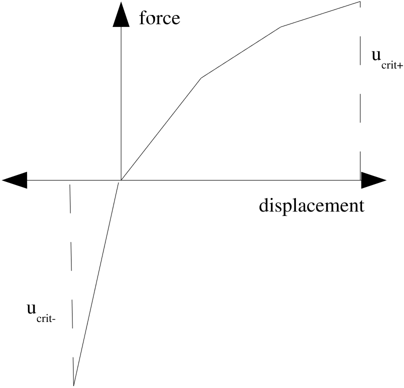(a) Normal force.

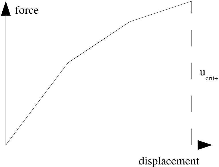(b) Tangential force.

Fig. 7.8 Spot weld force-displacement curves.

The sign of the normal displacement of the spot weld (generally tension at positive displacement or compression at negative displacement) is determined by the relative motion of the attached node and face as well as the normal direction of the face; see Fig. 7.9. Relative motion of the face along the face normal causes compressive spot weld response, while relative motion of the face opposite to the face normal leads to tensile spot weld response.

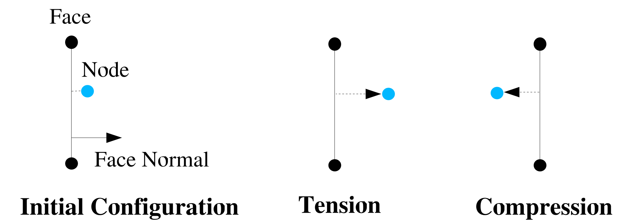
Fig. 7.9 Sign convention for spot weld normal displacements.

The attachment is defined between a node on one surface and the closest point on an element face on the other surface. Since a face is used to define one of the attachment points, it is possible to compute a normal vector and a tangent vector associated with the face. This allows resolution of displacement (distance, both positive and negative) and force (both tensile and compressive) into normal and tangential components.

Note that the direction vector used to decompose normal and tangential deformations in the weld is the current normal of the face associated with the spot weld. See Fig. 7.10 for a depiction of how normal and tangential displacements are computed in the spot weld. The spot weld deformation is decomposed into into normal (SW_ND) and tangential (SW_TD) components.

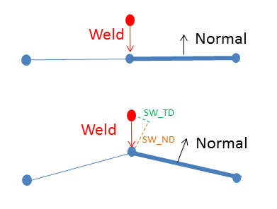
Fig. 7.10 Spot weld normal and tangent.

With normal and tangential vectors associated with the attachment, the attachment can be characterized for the case of pure tension and pure shear. The pure tensile and pure shear response of the spot weld will be governed by the input force/traction – displacement functions. Adagio includes two mechanisms for determining failure for cases that fall between pure tension and pure shear. In the first case, failure is governed by the equation

(7.4)\[(u_n/u_{n_{crit}})^p + (u_t/u_{t_{crit}})^p >= 1.0.\]

In (7.4), the distance from the node to the original attachment point on the face as measured normal to the face is \(u_n\), which is defined as the normal distance. The maximum value given for \(u_n\) in the normal displacement curve is \(u_{n_{crit}}\), but is different for positive and negative displacements. In Fig. 7.8(a), the value used for \(u_{n_{crit}}\) is \(u_{crit+}\) in the positive direction and \(u_{crit-}\) in the negative direction. The distance from the node to the original attachment point on the face as measured along a tangent to the face is \(u_t\), which is defined as the tangential distance. The maximum value given for \(u_t\) in the tangential displacement curve is \(u_{t_{crit}}\). The value \(p\) is a user-specified exponent that controls the shape of the failure surface.

Alternatively, Adagio permits a user-specified function to determine the failure surface. The function defines the ratio of \(u_t/u_{t_{crit}}\) at which failure will occur as a function of \(u_n/u_{n_{crit}}\). The function must range from 0.0 to 1.0, and have a value of 1.0 at 0.0 and a value of 0.0 at 1.0. These restrictions preserve proper failure for the cases of pure tension and pure shear.

To use the spot weld option in Presto, a SPOT WELD command block begins with the input line:

BEGIN SPOT WELD

and is terminated with the input line :

END [SPOT WELD]

A set of element faces which define one side of the spot weld (denoted the first surface) is specified with the SURFACE or ASSEMBLY SURFACE command line. The SURFACE command line can list one or more surfaces, while the ASSEMBLY SURFACE command line can list one or more assemblies of surfaces. Any surface listed on the SURFACE command line or contained in an assembly in ASSEMBLY SURFACE can be deleted from the list of surfaces by using a REMOVE SURFACE command line

When a spot weld is defined by a node set using a NODE SET|NODESET|ASSEMBLY NODE SET command line and a surface, the spot weld normal and tangential displacement functions define force/displacement relations. Alternatively a spot weld can be defined by a surface and a SECOND SURFACE command line. When a spot weld is defined by two surfaces the normal and tangential displacement functions define traction/displacement relations. A spot weld command block must include either a NODE SET|NODESET|ASSEMBLY NODE SET command line or a SECOND SURFACE command line but not both. In either case the faces used for the spot weld constraints are always defined by the SURFACE|ASSEMBLY SURFACE command line.

For the NODE SET|NODESET|ASSEMBLY NODE SET surface spot weld, each node in NODE SET|NODESET|ASSEMBLY NODE SET will look for a nearby face in SURFACE|ASSEMBLY SURFACE. If a sufficiently close face is found a spot weld will be created between the node and face using the force/displacement relations defined by the force and normal displacement curves. For the SECOND SURFACE surface spot weld each node in SECOND SURFACE will look for a nearby face in SURFACE|ASSEMBLY SURFACE. If a sufficiently close face is found a spot weld will be created between the node and the face. The node face relation will use a force/displacement relation defined by multiplying the weld displacement function (assumed to be a traction/displacement relation) by the tributary surface area of the node to compute a force/displacement function unique to that particular node. Thus the total max force resisted by a NODE SET|NODESET|ASSEMBLY NODE SET based weld is the number of nodes in the set times the maximum value of the provided force displacement curve. The total max force resisted by a SECOND SURFACE based weld is the tributary surface area of the second surface times the maximum value of the provided traction/displacement curve.

The normal force/traction–displacement curve is specified by a function named by the string function_nor_disp in the NORMAL DISPLACEMENT FUNCTION command line. The last points in the positive and negative directions are used as the displacements beyond which the spot weld fails. This function can be scaled by the real value scale_nor_disp in the NORMAL DISPLACEMENT SCALE FACTOR command line. The scaling factor scales the \(y\) values (force/traction) of the normal displacement function. Thus a scaling factor of 2.0 would indicate that for a given displacement the spot weld has twice the force defined in function_nor_disp. The default scale factor is 1.0.

The tangential force/traction–displacement curve is specified by a function named by the string function_tang_disp in the TANGENTIAL DISPLACEMENT FUNCTION command line. The last point in the positive direction in the tangential curve is used as the displacement beyond which the spot weld fails. This function can be scaled by the real value scale_tang_disp given in the TANGENTIAL DISPLACEMENT SCALE FACTOR command line; the default for this factor is 1.0. As with the normal displacement functions the scaling factors apply to the \(y\) value (force/tractions) used by the spot weld.

The failure surface between pure tension and pure shear is controlled by specifying either the failure envelope exponent, \(p\) in (7.4), or a failure function. The failure exponent is specified by the real value exponent in the FAILURE ENVELOPE EXPONENT command line. The failure function is specified by the FAILURE FUNCTION command line. If both a failure function and a failure exponent are given, then the failure function is used.

For an explicit transient dynamics, it is better to remove the force for the spot weld over several load steps rather than over a single load step once the failure criterion is exceeded. The FAILURE DECAY CYCLES command line controls the number of load steps over which the final force is removed (default value is 10). To remove the final force at a spot weld over five time steps, the integer specified by number_decay_cycles would be set to 5. Once the force at the spot weld is reduced to zero, it remains zero for all subsequent time (despite the function definition). That is, once a weld has reached the failure displacement, it will forever after be broken and will not reconnect if the node and face later move together again.

The user must set a tolerance for the node-to-face search with the

SEARCH TOLERANCE = <real>search_tolerance

command line. The value selected for search_tolerance will depend upon the distance between the nodes and surfaces used to define the spot weld.

If the user sets IGNORE INITIAL OFFSET = YES, the initial distance between the node and the face will be taken as the zero normal displacement distance for the spot weld. When using the IGNORE INITIAL OFFSET = YES command the initial normal force in the will be the value of the force-displacement curve at displacement=zero. The sign convention used to determine if a spot weld is in compression or tension is the same as without using IGNORE INITIAL OFFSET = YES as shown Fig. 7.11.

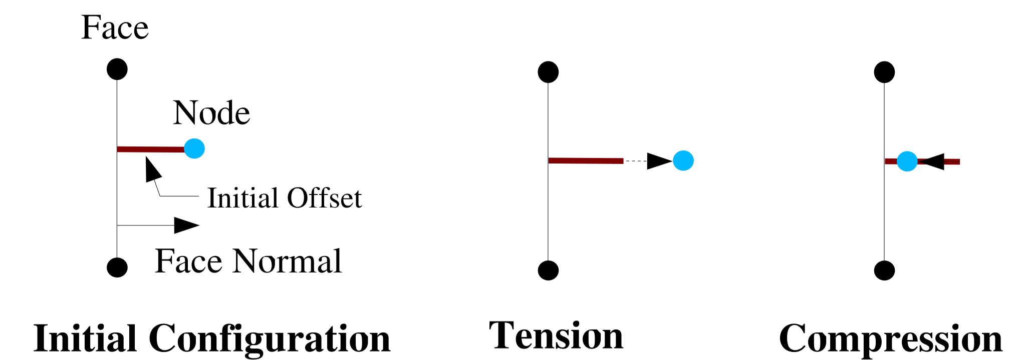
Fig. 7.11 Sign convention for spot weld normal displacements with IGNORE INITIAL OFFSET = YES.

The ACTIVE PERIODS and INACTIVE PERIODS command lines are used to activate or deactivate the boundary condition for certain time periods. See Section 2.6 for more information.

The CREATE VISUALIZATION ELEMENTS command line triggers the creation of beam elements to visualize the spot weld in output. These elements are for visualization purposes only and have no effect on the spot weld behavior. The default value is OFF. Each beam element is drawn between the welded node and the corresponding contact point on the welded surface.

Some special output data can be obtained from spot welds. The list of available output variables is documented in Table Table 9.9.

7.16.3.1. Spot Weld Limitations and Usage Guidelines

Warning

In explicit dynamics, spot welds do not inherently have an element critical time step because they have zero mass. However, spot welds may still decrease the global system time step. When spot welds with high stiffness relative to their attached elements are used in the model, the default element-based critical time step estimate may lead to instability in the spot weld.

When a node-based time step estimate is used, spot welds contribute their stiffness to the nodes associated with the spot weld, thus influencing the nodal time step (see Section 3.2.3.1). Thus, the node-based time step should remain stable, even in the presence of a stiff spot weld.

The spot weld stiffness is calculated conservatively as the sum of the current derivatives of the normal and tangential force functions. If the nodes attached to an element that governs the critical time step have spot weld stiffness contributions, log file output will indicate the approximate percentage reduction in the critical time step due to the spot weld stiffness contribution.

Warning

If the offset between the spot weld node and the attached face becomes large, the weld may be become unstable. This instability is related to potentially inconsistent handling of moments induced by weld forces acting over a finite gap. It is recommended that the normal gap offset between the spot weld node and the spot weld face not exceed roughly one-half of the characteristic element length in the neighboring mesh. Note that a large gap in either initial or deformed coordinates are both problematic. Thus, welds that can undergo large normal displacements prior to breakage may encounter stability problems once the normal gap in the weld is large.

If spot welds are used to represent bolts that are larger than the mesh size, it is recommended to use rigid patches on both sides of the interface. Rigid patches prevent concentrated forces and large deformations at the spot weld attachment point, such as in Fig. 7.10. Spot welds attached to rigid patches will also exhibit enhanced stability, for instance, under mesh refinement, since the characteristic face size is bound by the rigid patch size rather than the size of an individual face.

Warning

Although the spot weld is available for implicit computations, this use case is considered less mature than the explicit use case. Spot welds may adversely affect the conditioning of the linear systems solved in implicit analyses, and as a result can lead to poor convergence behavior.

Known Issue

Use of SECOND SURFACE is less mature and reliable than using NODE SET|NODESET. Instead of using a second surface, it is better to create a node set containing all the nodes of the desired surface.

Some other recommendations when using spot welds:

• When using node sets, be aware that the force will be distributed among all the nodes of the set. The distribution will also be uneven among the nodes which can cause failure of the spot weld due to concentrations of force on a particular node. If there is unexpected behavior, try starting with node sets that have only one node to better control the forces.

• If possible, use rigid surfaces for the surface and node set. This significantly improves behavior.

• The choice of SEARCH TOLERANCE greatly affects the performance of the spot weld. The value should be between 0 and the surface size, but probably no more than 25 percent of the length of the surface’s largest characteristic length. In general, select the largest in a range of reasonable values.

7.16.3.2. Example

The following is an example of a basic spot weld defined between the nodes of nodelist_17 and the faces of surface surface_3. Note the spot weld has a stiffness of \(500\times10^2\) in compression, a stiffness of \(100\times10^2\) in tension, and a stiffness of \(50\times10^2\) in shear. Once either the normal or tangential displacement in the weld reaches a value of approximately \(1.0\times10^{-2}\), the weld will fracture.

BEGIN FUNCTION spot_norm
  TYPE = PIECEWISE LINEAR
  BEGIN VALUES
    -1.0e-2 -500.0
     0.0       0.0
     1.0e-2  100.0
  END
END

BEGIN FUNCTION spot_tang
  TYPE = PIECEWISE LINEAR
  BEGIN VALUES
     0.0e-2   0.0
     1.0e-2  50.0
  END
END

BEGIN SPOT WELD
  NODE SET = nodelist_17
  SURFACE = surface_3
  NORMAL DISPLACEMENT FUNCTION = spot_norm
  TANGENTIAL DISPLACEMENT FUNCTION = spot_tang
  SEARCH TOLERANCE = 1.0e-3
END

7.16.4. Line Weld

BEGIN LINE WELD
  SURFACE|SIDESET|SIDE SET = <string list> surface_names
  REMOVE SURFACE = <string list> surface_names
  BLOCK = <string list> block_names
  ASSEMBLY BLOCK = <string list> assembly_names
  ASSEMBLY SURFACE = <string list> assembly_names
  REMOVE BLOCK = <string list>block_names
  SEARCH TOLERANCE = <real>search_tolerance
  FORMULATION = LINEAR|COROTATIONAL
  R DISPLACEMENT FUNCTION = <string>r_disp_function_name
  R DISPLACEMENT SCALE FACTOR = <real>r_disp_scale
  S DISPLACEMENT FUNCTION = <string>s_disp_function_name
  S DISPLACEMENT SCALE FACTOR = <real>s_disp_scale
  T DISPLACEMENT FUNCTION = <string>t_disp_function_name
  T DISPLACEMENT SCALE FACTOR = <real>t_disp_scale
  R ROTATION FUNCTION = <string>r_rotation_function_name
  R ROTATION SCALE FACTOR = <real>r_rotation_scale
  S ROTATION FUNCTION = <string>s_rotation_function_name
  S ROTATION SCALE FACTOR = <real>s_rotation_scale
  T ROTATION FUNCTION = <string>t_rotation_function_name
  T ROTATION SCALE FACTOR = <real>t_rotation_scale
  FAILURE ENVELOPE EXPONENT = <real>k(2.0)
  FAILURE DECAY CYCLES = <integer>number_decay_cycles
  REMOVE NODES FROM CONTACT = NONE|ALL|INTERACTION
  THROW ERROR|WARNING(ERROR) IF NO CONSTRAINTS ARE FOUND
  ACTIVE PERIODS = <string list>period_names
  INACTIVE PERIODS = <string list>period_names
  GAP REMOVAL = OFF|ON (OFF)
  DEBUG OUTPUT LOCAL COORDINATE SYSTEM
END LINE WELD

Warning

If a function provided by a R DISPLACEMENT FUNCTION, S DISPLACEMENT FUNCTION, T DISPLACEMENT FUNCTION, R ROTATION FUNCTION command does not have a maximum x-limit (e.g., constant and analytic functions), then the line weld will not fail for displacements or rotations in that direction.

The line weld capability is used to weld the edge of a shell to the face of another shell. The bond can transmit both translational and rotational forces. When failure of the line weld occurs, it breaks and no longer transmits any forces.

The edge of the shell that is tied to a surface is modeled with a block of one-dimensional elements (truss, beam, spring, etc.). The edge of the shell and the one-dimensional elements will share the same nodes. We will refer to the shell edge and the one-dimensional elements associated with it as the one-dimensional part of the line weld model. The element blocks with the one-dimensional elements are specified by using the BLOCK|ASSEMBLY BLOCK command line. More than one element block or assemblies of element blocks can be listed on this command line. The element blocks referenced by the BLOCK|ASSEMBLY BLOCK command line must be one-dimensional elements—truss, beam, spring, etc.

The other part of the line weld is a set of faces defined by shell elements; this set of faces is the two-dimensional part of the line weld. The surface (the two-dimensional part of the model) to which the nodes (from the one-dimensional part of the model) are to be bonded is defined by any surface of element faces derived from shell elements. The line weld will bond each node in the element blocks listed or contained in the assemblies listed in the BLOCK|ASSEMBLY BLOCK command line to the closest face (or faces) of element faces in the surfaces listed or contained in the assemblies listed in the SURFACE|ASSEMBLY SURFACE command line. More than one surface or assemblies of surfaces can be listed on this command line.

The command line SEARCH TOLERANCE sets a tolerance on the search for node-to-face interactions. For a given node, only those faces within the distance set by the search_tolerance parameter will be searched to determine whether the node should be welded to the face.

The line command FORMULATION specifies which line weld formulation to use: LINEAR or COROTATIONAL. The LINEAR formulation simply computes a gap between the beam nodes and the shell faces of the line weld. Then, this gap is used to compute the line weld deformation. For line welds with no initial gap, this formulation works well and is the most efficient.

The COROTATIONAL formulation is mostly for line welds that have initial gaps between the beam nodes and the shell faces. In this formulation, an RMSD (root mean squared distance) calculation is performed on all of the nodes involved in the line weld interaction. After performing the RMSD calculation, a rotation matrix is formed, and the initial gap vector is rotated into the current configuration. Then, the node-face gap is computed in the current configuration once again, and the difference between the current gap and the rotated model gap is the current deformation of the line weld.

Each section of the line weld has its own local coordinate system (\(r\), \(s\), \(t\)). Line welds are constructed via a node-face search. The search is performed from the nodes in the beam to the faces in the sideset. The \(r\)-direction lies along the beam element. The \(t\)-direction is orthogonal to the \(r\)-direction and normal to the face the node is projected to. The \(s\)-direction is the cross product between the \(r\)-direction and \(t\)-direction.

Force-per-unit-length-vs-displacement functions may be specified for all axes in the local coordinate system. Moment-per-unit-length-vs-rotation functions may also be specified for the all rotational direction, where rotations are in radians. All displacement functions are required to be specified; only the \(r\)-rotational stiffness is required for the rotational directions. SIERRA_CONSTANT_FUNCTION_ZERO can be used to give a zero stiffness. The functions only evaluate on the positive side and the relationship is assumed to be symmetric in compression versus tension.

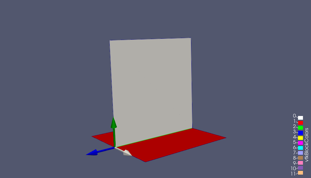
Fig. 7.12 Line Weld local coordinate system. The \(r\)-direction is blue, the \(s\)-direction is grey, and the \(t\)-direction is green.

The force-per-unit-length-vs-displacement function in the \(r\)-direction represents shear resistance in the direction of the weld; this function is specified by a SIERRA function name on the R DISPLACEMENT FUNCTION command line. The force-per-unit-length-vs-displacement in the \(s\)-direction represents shear resistance tangential to the weld; this function is specified by a SIERRA function name on the S DISPLACEMENT FUNCTION command line. The force-per-unit-length-vs-displacement in the \(t\)-direction function represents tearing resistance normal to the surface; this function is specified by a SIERRA function name on the T DISPLACEMENT FUNCTION command line. The moment-per-unit-length-vs-rotation about the \(r\)-axis represents a rotational tearing resistance; this is specified by a SIERRA function name on the R ROTATION FUNCTION command line, where rotations are in radians. Moment-per-unit-length-vs-rotation may also be specified for the \(s\) and \(t\)-axis as well via S ROTATION FUNCTION and T ROTATION FUNCTION command lines. Note, the \(s\) and \(t\) rotation specification is optional. Each SIERRA function used in this command block is defined via a FUNCTION command block in the SIERRA scope.

Any of the above functions can be scaled by using a corresponding scale factor. For example, the force-per-unit-length-vs-displacement function on the R DISPLACEMENT FUNCTION command line can be scaled by the parameter r_disp_scale on the R DISPLACEMENT SCALE FACTOR command line. The force-per-unit-length values of the force-per-unit-length-vs-displacement curve will be scaled; the displacement values are not scaled.

The failure for the line weld is similar to that for the spot weld. Denote the displacement or rotation associated with a line weld as \({\rm{\delta }}\). Suppose that \({\rm{\delta }}_i\) is a displacement in the \(r\)-direction. The force-per-unit-length-vs-displacement curve specified on the R DISPLACEMENT FUNCTION command line has a maximum displacement value \({\rm{\eta }}\). This is the maximum displacement the weld can endure in the \(r\)-direction before breaking. Associate this value of \({\rm{\eta }}\) with \({\rm{\delta }}_i\) by designating it as \({\rm{\eta }}_i\). Repeat this pairing process for all the displacements and the rotation \(r\) defining the line weld. Each displacement component in the line weld will be paired with one of the three maximum displacement values associated with the line weld. The \(r\) rotation component in the line weld will be paired with the maximum rotation value in the R ROTATION FUNCTION. Currently, the line weld is unable to fail in the \(s\) and \(t\) rotational directions. Note that if a function provided by a R DISPLACEMENT FUNCTION, S DISPLACEMENT FUNCTION, T DISPLACEMENT FUNCTION, or R ROTATION FUNCTION command does not have a maximum x-limit (e.g., constant and analytic functions), then the line weld will not fail for displacements or rotations in that direction.

The weld breaks under the following condition:

(7.5)\[\sqrt[k]{{\sum {\left( {\frac{{{\rm{\delta }}_i }}{{{\rm{\eta }}_i }}} \right)^k } }} > 1 .\]

In the above equation, the parameter \(k\) is set by the user. A typical value for \(k\) is 2. The summation takes place over all the failure functions (force-per-unit-length-vs-displacement and moment-per-unit-length-vs-rotation) for all the nodes. The value for \(k\) is specified on the FAILURE ENVELOPE EXPONENT command line.

For an explicit, transient dynamics analysis, it is better to remove the forces for the line weld over several time steps rather than over a single time step once the failure criterion is exceeded. The FAILURE DECAY CYCLES command line controls the number of time steps over which the final force is removed. To remove the final force at a line weld over five time steps, the integer specified by number_decay_cycles would be set to 5. Once the force in the line weld is reduced to zero, it remains zero for all subsequent time. Note, the line weld forces during the failure decay are independent of the line weld displacements or rotation and simply linearly decay from the force and moments reached at failure to zero over the specified number_decay_cycles.

The REMOVE NODES FROM CONTACT line command specifies if the nodes of the line weld should be removed from contact. This is often necessary due to the lofted geometry that is constructed for contact with lofted shells. If the ALL option is used, the nodes are completely removed from every interaction of contact. If the INTERACTION option is used, contact is only disallowed on specific interactions who have the same value of the SKIP_INTERACTION nodal field. Thus, if the beam nodes are specified in a SIDE_A contact surface, and the face nodes are specified in a SIDE_B contact surface, contact will be disallowed between these nodes and faces. If the NONE option is used, contact is allowed on all nodes of the line weld.

The default response if no constraints are found between the BLOCKS and SURFACES is to error allowing the user to remove or fix the boundary condition that is not being applied. If the user wants to bypass the error message they can turn it into a warning using THROW WARNING IF NO CONSTRAINTS ARE FOUND.

The ACTIVE PERIODS and INACTIVE PERIODS command lines provide an additional option for this boundary condition. These command lines are used to activate or deactivate the boundary condition for certain time periods. See Section 2.6 for more information about these command lines.

For line welds with offsets, it is recommended to use the option GAP REMOVAL = ON. This option can fix commonly observed robustness issues. The nodes on the beam of the offset line weld are moved to the matching face (found via contact search). Note, gap removal is OFF by default (different from SD, where gap removal is ON by default). A warning is triggered if an offset line weld is used without gap removal.

The local coordinate system created for each line weld may be visualized via the DEBUG OUTPUT LOCAL COORDINATE SYSTEM line command. If this line command is specified, the local coordinate system vectors will be output as a nodal variable on the nodes of the beam element. The fields created will be named: <line_weld_name>_r_dir, <line_weld_name>_s_dir, <line_weld_name>_t_dir.

Some special output data can be obtained from line welds. The list of available output variables is documented in Tables Table 9.10 and Table 9.24.

Warning

In explicit dynamics, line welds do not inherently have an element critical time step because they have zero mass. However, line welds may still decrease the global system time step. When line welds with high stiffness relative to their attached elements are used in the model, the default element-based critical time step estimate may lead to instability in the line weld.

7.16.5. Shell Solid Joint

BEGIN SHELL SOLID JOINT
  # block of shell elements
  BLOCK = <string list>block_names
  # Set of solid nodes
  NODE SET = <string list>nodelist_names
  ASSEMBLY BLOCK = <string list>assembly_names
  ASSEMBLY NODE SET = <string list>assembly_names
  SEARCH TOLERANCE = <real>tol
  TRUE GAUGE TEST = OFF|ON(OFF)  #EXPERIMENTAL DO NOT USE
  SIDE A SELECTION = NORMAL PROJECTION|
    NEAREST NODE(NORMAL PROJECTION)
  FOLLOW THICKNESS CHANGE = OFF|ON (OFF)
  ROTATION UPDATE TYPE = REISSNER|KIRCHHOFF (REISSNER)
  MEAN QUADRATURE ROTATION = OFF|ON (OFF)
END [SHELL SOLID JOINT]

The shell solid joint capability connects a set of solid nodes to a shell element block. Typically it is used to connect the nodes on the surface of a high-fidelity solid element block to the edge of a low-fidelity shell element block.

A shell solid joint enforces that the translations of the solid nodes remain compatible with the shell translations and rotations at the interface. The solid nodes will conform to the shell kinematic assumptions (e.g., plane sections remain plane) as if embedded in the shell. The through-thickness thinning or expansion of the solid mesh in the joint region is constrained by the thickness change of the shells. The shell solid joint constraint equations are written at the solid nodes, i.e., they constrain each solid node within search tolerance to a single shell element.

The BLOCK|ASSEMBLY BLOCK commands select one or more sets of shell elements to constrain the solid nodes to. These must be two dimensional shell – not membrane – formulation elements. The NODE SET|ASSEMBLY NODE SET commands select a set of nodes to constrain to the shells. These may be nodes connected to any type of solid element (i.e., they should not have rotational degrees of freedom).

The SEARCH TOLERANCE command optionally sets the tolerance for how close nodes need to be to shells to become constrained. If the SEARCH TOLERANCE command is not used a search tolerance is selected automatically based on the shell thickness, lofting factor, and in-plane size. The automatic search tolerances are set such that the joint will constrain any solid node found within or nearby the volumetric domain occupied by the theoretical shell material. A pictorial representation of how search tolerances are used is shown in Fig. 7.13.

The TRUE GAUGE TEST option is experimental and should not be used.

The SIDE A SELECTION command is used to change how the constrained nodes are projected to the plane of the shell. By default the constraint is made via a projection of the node along the shell normal onto the plane of the shell. The NEAREST NODE option will instead project the constrained node to the nearest node on the shell. The NEAREST NODE option can potentially be useful when the shell and solid meshes have been constructed contiguously such that a line of nodes on the solid side directly one to one maps to a single node on the shell side. For such a case use of the NEAREST NODE option will remove any possibility of mapping errors due to shell warping or curvature. However, the default NORMAL PROJECTION option should always be used for all general or non-matching shell and solid meshes.

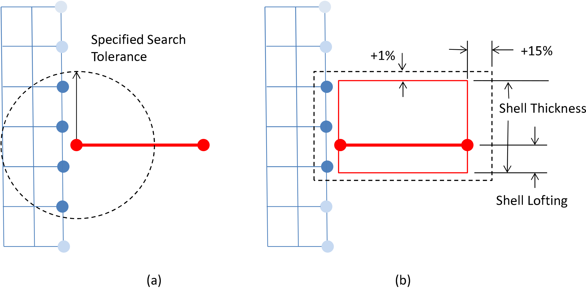
Fig. 7.13 Search tolerances for shell-solid joints. (a) input; (b) automatic.

7.16.5.1. Shell Solid Joint in Implicit Computations

Warning

Although the shell solid joint is available for implicit computations, this use case is considered experimental. There are many known issues with the implicit shell solid joint, leading to poor convergence in serial analyses and potential inconsistencies in parallel analyses.

A number of implicit-specific options exist for the shell solid joint.

The shell solid joint constraint is enforced through the control contact multilevel solver in implicit analyses. Thus, a CONTROL CONTACT solver block must be present in the solver settings.

By default the movement of the solid modes on the interface interface is uncoupled to any Poisson thinning or thickening of the attached shell. The FOLLOW THICKNESS CHANGE = ON option will turn on coupling of this degree of freedom ensuring that the solid nodes move up or down the shell normal consistently with the shell thickness changes. This option can potentially lead to a more accurate coupling of the joint during large membrane stretching. However, the coupling may also in some circumstances over constrain the joint causing robustness issues.

The ROTATION UPDATE TYPE command defines how shell solid joints computes coupling rotations. The default REISSNER option couples rotations to the rotational degrees of freedom of the shell nodes. The KIRCHHOFF option couples rotations to changes in shell element normal. Generally both options should yield the similar results. The KIRCHHOFF option could in some cases produces a stiffer but more stable result. This stability can be particular important if constraining a stiff material shell to a soft material solid.

The MEAN QUADRATURE ROTATION command allows tying rotations to the average shell rotation (ON) option rather than the nodal point (default OFF) option. This command has a similar effect to the ROTATION UPDATE TYPE where the ON option can create a potentially stiffer but more stable joint.

7.16.5.2. Restrictions and Assumptions

The following guidelines apply to both the explicit and implicit shell solid joint.

• Though the shell solid joint is a kinematic MPC, it can potentially artificially stiffen the nearby elements and thus it may be necessary to manually reduce the analysis time step a small amount to ensure integration stability.

• It is generally assumed that there are minimal or no lateral gaps or overlaps in the joint. Gaps or overlaps between the shell block(s) and solid(s) will tend to introduce additional artificial stiffness into the joint.

• Any offset between the solid cross-section neutral bending plane and the shell midplane will result in an effective lofting distance, which may increase the stiffness of the structure unexpectedly. (This is because the enforcement of shell kinematics on the solid nodes forces the solid to rotate and bend around the shell midplane as if part of the shell.)

• In order to correctly enforce moment and rotation compatibility across the joint, the joint must contain at least two solid nodes in the shell normal (i.e., thickness) direction. It is preferable to have five or more solid nodes in the shell normal direction for a smoothly connected joint.

• For best results the solid side of the joint should be meshed as fine or finer than the shell side. A finely meshed shell connected to a coarsely meshed solid will result in constraints at only the solid nodes, leading to unconstrained shells nodes at the joint.

• The shell solid joint constraint can constrain each solid node to only one shell. In ambiguous cases the “best” matching shell will be selected based on proximity.

• Care should be taken if using the shell solid joint on the same part of a mesh as contact or other kinematic or rigid body constraints. If multiple constraint types come into conflict generally either one of the constraints sets will not be enforced or stability problems will result.

7.16.6. Viscous Damping

BEGIN VISCOUS DAMPING <string>damp_name
  #
  # block set commands
  BLOCK = <string list>block_names
  ASSEMBLY = <string list>assembly_names
  INCLUDE ALL BLOCKS
  REMOVE BLOCK = <string list>block_names
  #
  MASS DAMPING COEFFICIENT = <real>mass_damping
  ROTATIONAL MASS DAMPING COEFFICIENT = <real>rot_mass_damping
  STIFFNESS DAMPING COEFFICIENT = <real>stiff_damping
  #
  VELOCITY DAMPING COEFFICIENT = <real>damping_coefficient
  VELOCITY DAMPING FUNCTION = <string>function_name
  #
  RIGID BODY INVARIANCE = OFF|ON(OFF)
  #
  # additional commands
  ACTIVE PERIODS = <string list>period names
  INACTIVE PERIODS = <string list>period_names
END [VISCOUS DAMPING <string>damp_name]

The VISCOUS DAMPING command block adds simple Rayleigh viscous damping to mesh nodes. At each node, Presto computes a damping coefficient, which is then multiplied by the node velocity to create a damping force. The damping coefficient is the sum of the mass times a mass damping coefficient and the nodal stiffness times a stiffness damping coefficient. In general, the mass damping portion damps out low-frequency modes in the mesh, while the stiffness damping portion damps out higher-frequency terms. Appropriate values for the damping coefficients depend on the frequencies of interest in the mesh. The general expression for the critical damping fraction, \(c_{d}\), for a given frequency is

(7.6)\[c_{d} = \frac{1}{2}\left( k_{d} \omega + \frac{m_{d}}{\omega} \right)\, ,\]

where \(k_{d}\) is the stiffness damping coefficient, \(m_{d}\) is the mass damping coefficient, and \(\omega\) is the frequency of interest. The stiffness damping portion must be used with caution. Because this term depends on the stiffness, it can affect the critical time step. Thus certain ranges of values for the stiffness damping coefficient can change the critical time step for the mesh. As Presto does not currently modify the critical time step based on the selected values for this coefficient, some choices for this parameter can cause solution instability.

Velocity damping applies forces that, in the absence of other forces, have the effect of directly opposing nodal velocity according to the expression

(7.7)\[\mathbf{v}_{new} = (1.0-v_{d}) \mathbf{v}_{old} ,\]

where \(v_{d}\) is the velocity damping coefficient and \(\mathbf{v}\) represents the velocity. That is, the coefficient \(v_{d}\) represents the fraction by which the previous nodal velocity will be reduced by the applied damping forces in the absence of other forces.

7.16.6.1. Block Set Commands

The block set commands portion of the VISCOUS DAMPING command block defines a set of element blocks associated with the viscous damping and can include some combination of the following command lines:

BLOCK = <string list>block_names
ASSEMBLY = <string list>assembly_names
INCLUDE ALL BLOCKS
REMOVE BLOCK = <string list>block_names

These command lines provide a set of Boolean operators for constructing a set of element blocks. See Section 7.1.1 for more information about the use of these command lines for creating a set of element blocks used by viscous damping. There must be at least one BLOCK, ASSEMBLY, or INCLUDE ALL BLOCKS command line in the command block. All the nodes associated with the elements specified by the block set commands will have viscous damping forces applied. Assemblies may contain blocks, or assemblies of these.

7.16.6.2. Viscous Damping Coefficient

The mass damping coefficient, \(m_d\), in (7.6) is specified using the parameter mass_damping on the command line:

MASS DAMPING COEFFICIENT = <real>mass_damping
ROTATIONAL MASS DAMPING COEFFICIENT = <real>rot_mass_damping

Note, the MASS DAMPING COEFFICIENT affects only translational degrees of freedom while the ROTATIONAL MASS DAMPING COEFFICIENT affects only the rotational degrees of freedom on shells, beams, and rigid bodies. Mass damping most strongly damps the low-frequency modes, and in Presto, is applied as a boundary condition which does not affect the critical time step.

The stiffness damping coefficient, \(k_d\), in (7.6), is specified as the parameter stiff_damping on the command line:

STIFFNESS DAMPING COEFFICIENT = <real>stiff_damping

Stiffness damping most strongly damps high-frequency modes and is applied through a stress correction of the pressure term at the element level. Because this type of damping is done at the element level, it has a direct effect on the critical time step as seen in (7.8), where \(\epsilon = \frac{k_d\omega}{2}:math:`in the absence of mass damping and `\frac{2}{\omega} \approx \frac{m}{\kappa}\).

(7.8)\[\Delta t \leq \frac{2}{\omega}\left ( \sqrt{1 + \epsilon^{2}} - \epsilon \right )\]

The velocity damping coefficient, \(v_d\), in (7.7), is specified by either the constant parameter vel_damping on the command line:

VELOCITY DAMPING COEFFICIENT = <real>vel_damping

or the user defined time-dependent function \(v_d(t)\) function_name on the command line:

VELOCITY DAMPING FUNCTION = <string>function_name

Velocity damping applies a damping term that has the effect of lowering velocity (the end result is described by (7.7)), and damping out all modes. Velocity damping is primarily used to drive a dynamic solution towards static equilibrium during or after a preload procedure.

Velocity damping and mass damping may not be used in combination.

A velocity damping coefficient and a velocity damping function may not be used in combination. The constant damping coefficient \(v_d\) or the damping function \(v_d(t)\) must be between 0 and 1:

(7.9)\[0 \leq v_d(t) \leq 1 \quad \textrm{for all } \; t\in \{t_s\}\]

where \(t \in \{t_s\}\) are actual simulation time steps. A velocity damping function that evaluates outside these bounds may result in analysis termination. Note that since arbitrary user-defined functions may depend on runtime solution variables, this check cannot be performed at parse time.

RIGID BODY INVARIANCE = OFF|ON(OFF)

By default mass and velocity damping apply a force to each node that opposes the current velocity of that node. This acts as if the part is moving through a viscous fluid. This force will damp out both vibration and net rigid body motions. The rigid body invariance option applies damping forces based on the difference between the node velocity and the net average velocity of the node set. The intent is to damp out vibrations in the part but not affect the net rigid body motions. Note, this option only makes sense if the damping is applied on contiguous parts. For example applying rigid body invariant damping to two pieces moving in opposite directions would still slow both parts as the net rigid motion of the parts moving away from one another is zero. An additional effect of the rigid body invariance = on option is that the net force and moment applied by viscous damping will be assured to be zero.

7.16.6.3. Additional Command

The ACTIVE PERIODS and INACTIVE PERIODS command lines can optionally appear in the VISCOUS DAMPING command block:

ACTIVE PERIODS = <string list>period_names
INACTIVE PERIODS = <string list>period_names

This command line can activate or deactivate the viscous damping for certain time periods. See Section 2.6 for more information about this command line.

7.16.7. Artificial Strain

BEGIN ARTIFICIAL STRAIN
  #
  # Zone of application commands
  INCLUDE ALL BLOCKS
  ELEMENT = <int list>elem_nums
  BLOCK = <string list>block_names
  ASSEMBLY = <string list>assembly_names
  REMOVE BLOCK = <string list>block_names
  #
  # Strain definition commands
  STRAIN TYPE = LOG|ENGINEERING(ENGINEERING)
  FUNCTION = <string>function_name
    [SCALE FACTOR = <real>scale]
  DIRECTION <string>dir_name FUNCTION = <string>dir_func
    [SCALE FACTOR = <real>scale]
  DIRECTION FIELD <string>field_name FUNCTION =
    <string>field_dir_func [SCALE FACTOR = <real>scale]
  R FUNCTION = <string>r_func [SCALE FACTOR = <real>scale]
  S FUNCTION = <string>s_func [SCALE FACTOR = <real>scale]
  T FUNCTION = <string>t_func [SCALE FACTOR = <real>scale]
END [ARTIFICIAL STRAIN]

A The ARTIFICIAL STRAIN command block defines an artificial strain applied on a block by block or element by element basis. Artificial strains may be useful for fitting parts together for a preload analysis or modeling a variety of other physics that could cause material expansion or contraction (such as radiation induced expansion, material desiccation, etc.)

Artificial strains may also be defined in the material block, see Section 5.1.3. However, defining artificial strains by boundary condition as shown in this section is more flexible.

A variety of commands can be used to describe the set of elements this command block applies to as detailed in Section 7.1.1.

Artificial strains may be applied based in either the LOG or ENGINEERING strain space as defined from the STRAIN TYPE command. There are several ways to define the applied strain tensor. One and only one of the following command sets may be used.

• FUNCTION is a single function defining the isotropic strain to apply. The function is a time history function optionally scaled by an input constant.

• DIRECTION may be used up to three times to define up to three orthogonal directions paired with separate time history functions in which to apply strain. The directions’ names used here are defined in a Sierra scope DIRECTION command. The direction command is generally only applicable to three dimensional elements and defines the strain directions in the global XYZ coordinate system. The functions may be optionally scaled by an input constant.

• DIRECTION FIELD may be used along with DIRECTION lines to define up to three orthogonal directions paired with separate time history functions in which to apply strain. The field names given to DIRECTION FIELD refer to name of an element direction variable. The element direction variable must be a defined element output field and must have exactly three components at each element. The direction field may be populated by a number of methods including USER OUTPUT to define the field on the fly or use of INITIAL CONDITION blocks to read the field from the mesh file. Note, though the field used can potentially vary in time the behavior of artificial strain is not well defined for time variant directions and it is recommended that only directions that are constant in time be used. Additionally at each and every element the set of up to three DIRECTION FIELD directions and DIRECTION directions must be orthogonal to each other. The functions may be optionally scaled by an input constant.

• the R, S, T FUNCTION commands define strain in the element local RST Section 6.2.5 coordinate system For solids this generally corresponds to the global XYZ coordinate system. For shells and membranes R and S are the in plane directions and T is the through thickness direction. For beams and trusses R is the axial direction and S and T are the lateral directions. These functions are time history functions and may be optionally scaled by an input constant.

Note, the artificial strain is not an absolute constraint. An element could be artificially shrunk and then stretched by actual material strain in a way that the element shape doesn’t change, but the element does accumulate stress and strain energy. If artificial strain is applied uniformly to an unconstrained body that strain will grow or shrink the body as described by the artificial strain in a nominally stress free manner.

7.16.7.1. Restrictions and Usage Guidelines

Artificial strain cannot be simultaneously defined in a material and in the artificial strain block for the same element. Thermal strain may be defined in a material and artificial strain in an artificial strain block. However, in such cases the strain must be of matching type (LOG or ENGINEERING.)

One common error is assuming strain applied in the direction (1, 1, 0) has the same effect of applying an equal R and S strain. Applying a strain in the direction of 1, 1, 0 expands the body uniformly along the 45 degree direction vector. Applying a strain in both the R and S directions expands the body uniformly in the RS plane.

It is possible to apply any arbitrary strain state by computing the eigenvectors and values of the strain state and then applying direction strains in the directions of the eigenvectors with the magnitudes of the eigenvalues.

Note, strains should generally be applied by functions that are smooth in time. A sharp jump in the target artificial strain over a time step will tend to produce a strong shock in the system.

Assemblies may contain blocks, or assemblies of these.

7.16.8. Tied Multi-Point Constraints

BEGIN TIED MPC
  #
  TIED FACES = <string list>BLOCKS/SURFACES/ASSEMBLIES
  TIED NODES = <string list>BLOCKS/SURFACES/NODE SETS/ASSEMBLIES
  #
  # Tied contact search commands
  SEARCH TOLERANCE =  AUTO|<real>tolerance (AUTO)
  VOLUMETRIC SEARCH TOLERANCE = <real>vtolerance
  SEARCH CONFIGURATION = MODEL|CURRENT (CURRENT)
  #
  # DOF subset selection
  COMPONENTS = X|Y|Z|RX|RY|RZ
  REMOVE NODES FROM CONTACT = NONE|ALL|INTERACTION
    REMOVE GAPS AND OVERLAPS = OFF|ON(OFF)
  THROW ERROR|WARNING(ERROR) IF NO CONSTRAINTS ARE FOUND
END [TIED MPC]

Sierra/SM provides a tied contact multi-point constraint (MPC) capability that allows a code user to tie a set of nodes to a set of faces. The BEGIN TIED MPC and BEGIN EQUATION MPC (see Section 7.16.9) command blocks replace the capabilities of BEGIN MPC (deprecated in the 4.56 release). For tied contact MPCs, a proximity search is performed to create a set of MPCs that act as tied contact constraints. If the MPCs are created in this way, the search is performed at the time of initialization to find pairings of nodes (defined from the TIED NODES command line) to faces (defined from the TIED FACES command line). TIED FACES may be names of blocks, assemblies of blocks or surfaces, and/or surfaces and TIED NODES may be names of blocks, surfaces, node sets, and/or assemblies of blocks, surfaces, or nodesets. A separate constraint is created for each node in the TIED NODES. This type of MPC is equivalent to using pure tied contact and is significantly faster than standard tied contact for explicit dynamics analyses.

SEARCH TOLERANCE =  AUTO|<real>tolerance (AUTO)

The SEARCH TOLERANCE command line specifies the maximum distance between a node and a face to create an MPC. This has a similar meaning to the search tolerance used in standard tied contact. By default, the search tolerance is set to AUTO which automatically computes the search tolerance value internally. The value that is computed as the search tolerance is 15 percent of the second smallest edge length of the face.

VOLUMETRIC SEARCH TOLERANCE = <real>vtolerance

In addition to creating node/face constraints, a search can be used to create volumetric constraints, in which nodes among the TIED NODES that are not within the SEARCH TOLERANCE of the TIED FACES will also be constrained if their distance from nodes on the TIED FACES is less than or equal to the VOLUMETRIC SEARCH TOLERANCE. A set of node/face constraints is first created for the TIED NODES within the standard search tolerance of any TIED FACES. Next, a volumetric constraint is created for any remaining unconstrained nodes within the VOLUMETRIC SEARCH TOLERANCE of nodes on the TIED FACES. Each volumetric constraint gets distance-weighted MPC contributions from the nodes of the TIED FACES that are within the search tolerance.

SEARCH CONFIGURATION = MODEL|CURRENT (CURRENT)

The configuration in which nodes are searched for to create the MPCs can be changed via the SEARCH CONFIGURATION command. This can be useful if a restart or procedural transfer is performed and the MPCs need to change or remain the same as the start of the simulation.

COMPONENTS = X|Y|Z|RX|RY|RZ

By default, tied multi-point constraints are applied to all degrees of freedom of the nodes involved. For nodes that only have translational degrees of freedom, all three components (X, Y and Z) are constrained. Likewise, for nodes that have both translational and rotational degrees of freedom, all six components (X, Y, Z, RX, RY and RZ) are constrained. The COMPONENTS command line can be used to enforce the constraint on a subset of the degrees of freedom. If the COMPONENTS command line is included in a TIED MPC command block, only the components listed would be constrained.

The REMOVE NODES FROM CONTACT line command specifies if interactions containing a node of the tied multi-point constraints (MPCs) should be removed from contact. The ALL option signals removal of all contact interactions containing an MPC node. The INTERACTION option restricts removal to contact interactions where the node pairing belongs to the same MPC. If all translational components are present, REMOVE NODES FROM CONTACT defaults to the INTERACTION option. In particular, this applies when no components are specified (since this implies all degrees of freedom are included) or if all translational components (X, Y, Z) are included in the COMPONENTS command. An illustration of the ALL, INTERACTION, and NONE options are shown in Fig. 7.14. The REMOVE NODES FROM CONTACT line command is valid in both explicit and implicit.

Alternative form of contact and MPC constraints If the REMOVE NODES FROM CONTACT command is not specified or is set to NONE and all components of an MPC are not constrained, MPCs are attempted to be handled in contact via an MPC friction model. In contact, nodes are identified that are both in contact interactions as well as defined in MPCs. After all other friction models have been enforced, the MPC friction model is run on the back end and attempts to remove all contact forces that are aligned with constrained MPC directions. This is due to the fact that MPCs have a higher constraint rank than contact (See D. Constraint Enforcement Hierarchy for more information regarding constraint rank information).

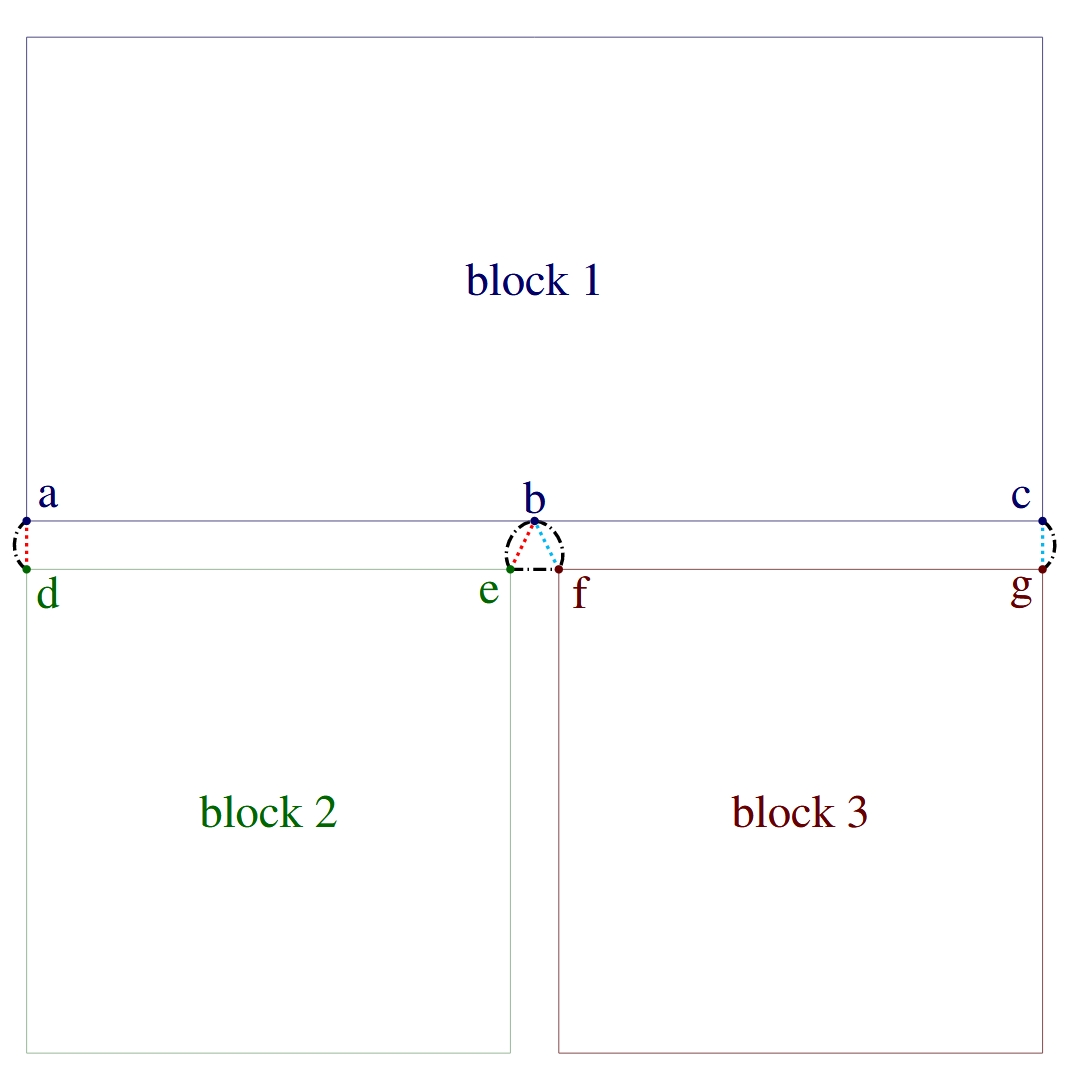
Fig. 7.14 Illustration of the command REMOVE NODES FROM CONTACT. In this example there are two MPCs, one between block 1 and block 2, represented with cyan dotted lines, and one between block 1 and block 3, represented with red dotted lines. The black dash dotted lines represent contact interactions. The NONE option deletes no interactions. The INTERACTION option deletes the contact interactions between node pairs (a,d), (b,e), (b,f), and (c,g), since each node pairing belongs to the same MPC. The ALL option additionally deletes the contact interaction between node pair (e,f) since both nodes $e$ and \(f\) are mpc nodes, despite not being in the same MPC.

To use tied MPCs, the TIED FACES and TIED NODES must be defined. It is important to note that the TIED FACES cannot contain any node sets or assemblies of node sets.

The following example demonstrates how to use Tied MPCs between two surfaces:

BEGIN TIED MPC
  TIED FACES = surface_10
  TIED NODES = surface_11
END MPC

The following example demonstrates the usage of Tied MPCs for both tied and volumetric constraints. Assuming that surface_10 is adjacent to the exterior surface of block_1, this command block would result in tied contact between the exterior nodes of block_1 and the faces of surface_10, and volumetric constraints between the interior nodes of block_1 and the exterior nodes of block_1.

BEGIN TIED MPC
  TIED FACES = surface_10
  TIED NODES = block_1
  VOLUMETRIC SEARCH TOLERANCE = 3.0
END MPC

Tied MPCs can potentially be in conflict with other constraints. Refer to D. Constraint Enforcement Hierarchy for information on how conflicting constraints are handled.

For a list of fields available for output, see Table Table 9.11.

7.16.8.1. Resolve Multiple MPCs

The behavior of tied multi-point constraints is ill-defined when a node within the TIED FACES is constrained to more than one set of nodes within TIED NODES. Sierra/SM’s tied MPC capability can handle chained MPCs, where a node in the TIED FACES is a node within the TIED NODES in another constraint, but it cannot simultaneously enforce multiple tied MPCs that have the same TIED FACES node.

RESOLVE MULTIPLE MPCS = ERROR|FIRST WINS|LAST WINS|ENFORCE ALL|
  IGNORE(ERROR)

The RESOLVE MULTIPLE MPCS command line, used within the region scope, controls how to resolve cases where a node within the TIED NODES is constrained to more than one set of nodes within the TIED FACES. Although multiple MPCs cannot be simultaneously enforced, this command provides ways to work around this problem that may be acceptable in many situations. The default option is ERROR, which results in an error message and terminates the code if this occurs. Alternatively, this command can take the following options:

• FIRST WINS Keep only the first MPC seen at a node (MPC order generally determined by input deck order).

• LAST WINS Keep only the last MPC seen at a node (MPC order generally determined by input deck order).

• ENFORCE ALL Attempt to simultaneously enforce all MPCs seen at a node. As long as the MPCs are orthogonal this may work. If the MPCs are not orthogonal this will likely lead to an erroneous result or stability issues.

• IGNORE If a node is found with multiple MPCs, ignore all the conflicting MPCs and enforce none.

7.16.8.2. Remove Gaps and Overlaps

Depending on how the model is constructed, there may be a gap between the TIED FACES and the TIED NODES in the initial configuration. Tied MPCs are best posed when this gap is zero. The option REMOVE GAPS AND OVERLAPS, if set to ON, moves the constrained node to the constraint point during initialization, explicitly zeroing the gap. The default value for this command is OFF.

7.16.8.3. Throw ERROR|WARNING If No Constraints Are Found

The default response if no constraints are found between the TIED FACES and the TIED NODES is to error allowing the user to remove or fix the boundary condition that is not being applied. If the user want to bypass the error message they can turn it into a warning using THROW WARNING IF NO CONSTRAINTS ARE FOUND.

7.16.9. Equation Multi-Point Constraints

BEGIN EQUATION MPC
  #
  # Equation MPC commands
  SIDE A NODE SET = <string list>side_a_nset
  SIDE A NODES = <integer list>side_a_nodes
  SIDE A WEIGHTS = <real list>side_a_weights
  SIDE A SURFACE = <string list>side_a_surf
  SIDE A BLOCK = <string list>side_a_block
  SIDE A ASSEMBLY = <string list>side_a_assembly
  SIDE B NODE SET = <string list>side_b_nset
  SIDE B NODES = <integer list>side_b_nodes
  SIDE B SURFACE = <string list>side_b_surf
  SIDE B BLOCK = <string list>side_b_block
  SIDE B ASSEMBLY = <string list>side_b_assembly
  #
  # DOF subset selection
  COMPONENTS = X|Y|Z|RX|RY|RZ
END [EQUATION MPC]

# Control handling of multiple MPCs
RESOLVE MULTIPLE MPCS = ERROR|FIRST WINS|LAST WINS|
                        ENFORCE ALL|IGNORE(ERROR)

Sierra/SM provides an equation multi-point constraint (MPC) capability that allows a code user to specify arbitrary constraints between sets of nodes. The BEGIN EQUATION MPC and BEGIN TIED MPC (see Section 7.16.8) command blocks replace the capabilities of BEGIN MPC (deprecated in the 4.56 release). The commands to define an equation MPC are all listed within a EQUATION MPC command block. The equation type of MPC imposes a constraint between a set of side A nodes and a set of side B nodes. The motion of the side B nodes is constrained to be equal to the average motion of the side A nodes. This type of MPC is most useful if there is either a single side A node and one or more side B nodes, or multiple side A nodes and a single side B node. If there are multiple side B nodes, they are constrained to move together as a set.

The sets of side A and side B nodes used in the MPC can be defined by using a node set on the mesh file, a list of nodes provided in the input file, or a surface on the mesh file from which a list of nodes is extracted. This can be done for the set of side A nodes using one or more of the following commands:

SIDE A NODE SET = <string list>side_a_nset
SIDE A NODES = <integer list>side_a_nodes
SIDE A SURFACE = <string list>side_a_surf
SIDE A BLOCK = <string list>side_a_block
SIDE A ASSEMBLY = <string list>side_a_assembly
SIDE A WEIGHTS = <real list>side_a weights
SIDE B NODE SET = <string list>side_b_nset
SIDE B NODES = <integer list>side_b_nodes
SIDE B SURFACE = <string list>side_b_surf
SIDE B BLOCK = <string list>side_b_block
SIDE B ASSEMBLY = <string list>side_b_assembly

The SIDE A NODE SET and SIDE B NODE SET command lines specify the names of node sets in the mesh file. The nodes in these node sets are included in the sets of side A or side B nodes for the constraint.

The SIDE A NODES and SIDE B NODES command lines specify lists of integer IDs of nodes to be included in the sets of side A or side B nodes for the constraint.

The SIDE A SURFACE and SIDE B SURFACE command lines specify the name of a surface in the mesh file. The nodes contained in this surface are included in the sets of side A or side B nodes for the constraint.

The SIDE A BLOCK and SIDE B BLOCK command lines specify the names of a block in the mesh file. The nodes contained in these blocks are included in the sets of side A or side B nodes for the constraint.

The SIDE A ASSEMBLY and SIDE B ASSEMBLY command lines specify the names of an assembly of blocks, surfaces, nodesets, or assemblies in the mesh file. The nodes contained in these blocks are included in the sets of side A or side B nodes for the constraint.

The SIDE A WEIGHTS command can be used to explicitly define a constraint equation. This command is subject to several restrictions. The SIDE A WEIGHTS command must be used with a SIDE A NODES command and cannot be used with a SIDE A NODE SET, SIDE A SURFACE, SIDE A BLOCK, or SIDE A ASSEMBLY command. If the SIDE A WEIGHTS is used the number number of weights must be the same as the number of nodes in the SIDE A NODES command. Negative weights are allowed. However, negative MPC weights can potentially cause stability problems in explicit analysis.

COMPONENTS = X|Y|Z|RX|RY|RZ

By default, multi-point constraints are applied to all degrees of freedom of the nodes involved. For nodes that only have translational degrees of freedom, all three components (X, Y and Z) are constrained. Likewise, for nodes that have both translational and rotational degrees of freedom, all six components (X, Y, Z, RX, RY and RZ) are constrained. The COMPONENTS command line can be used to enforce the constraint on a subset of the degrees of freedom. If the COMPONENTS command line is included in a EQUATION MPC command block, only the components listed would be constrained.

The following is an example of use of the SIDE A WEIGHTS command to define an equation MPC.

BEGIN EQUATION MPC
  SIDE B NODES    = 23
  SIDE A NODES   = 26    12   16
  SIDE A WEIGHTS = 0.5 0.25 0.25
  COMPONENTS = X
END MPC

The above MPC adds a constraint that the X displacement at node 23 will always be equal to 0.5 times the X displacement at node 26 plus 0.25 the X displacement at node 12 plus 0.25 the X displacement at node 16.

Equation MPCs can potentially be in conflict with other constraints. Contact interactions will be removed if both nodes belong to equation MPCs. This is because MPCs have a higher constraint rank than contact. Refer to D. Constraint Enforcement Hierarchy for information on how conflicting constraints are handled.

For a list of fields available for output, see Table Table 9.11.

7.16.9.1. Resolve Multiple MPCs

The behavior of multi-point constraints is ill-defined when a side A node is constrained to more than one set of side B nodes. Sierra/SM’s MPC capability can handle chained MPCs, where a side A node is a side B node in another constraint, but it cannot simultaneously enforce multiple MPCs that have the same side B node.

Refer to Section 7.16.8.1 for documentation of the RESOLVE MULTIPLE MPCS command line.

7.16.10. Submodel

BEGIN SUBMODEL
  #
  EMBEDDED BLOCKS = <string list>embedded_block
  EMBEDDED ASSEMBLIES = <string list>embedded_assembly
  ENCLOSING BLOCKS = <string list>enclosing_block
  ENCLOSING ASSEMBLIES = <string list>enclosing_assembly
END [SUBMODEL]

Sierra/SM provides a method to embed a submodel in a larger finite element model. The element blocks for both the submodel and the larger system model should exist in the same mesh file. The space occupied by the embedded blocks should also be occupied by the enclosing blocks.

This capability ties each node of the submodel to an element in the larger finite element model. The code makes no correction for mass due to volume overlap. However, this correction often can be done easily by hand simply by adjusting the density of the submodel block so that it is the difference between the density of the submodel block and the enclosing block.

Contact interactions will be removed if both nodes belong to a submodel. This is because submodels are treated as MPCs, which have a higher constraint rank than contact. Refer to D. Constraint Enforcement Hierarchy for information on how conflicting constraints are handled.

The embedded blocks (the submodel blocks), embedded assemblies of blocks (the submodel blocks), the enclosing blocks (the system model blocks), the enclosing assemblies of blocks (the system model blocks) are specified using the following four line commands:

EMBEDDED BLOCKS = <string list>embedded_block
EMBEDDED ASSEMBLIES = <string list>embedded_assembly
ENCLOSING BLOCKS = <string list>enclosing_block
ENCLOSING ASSEMBLIES = <string list>enclosing_assembly

For example, to embed block_7 and block_8 inside a system model where the embedded blocks are within block_2, block_3, and block_5, the following can be used:

BEGIN SUBMODEL
  EMBEDDED BLOCKS = block_7 block_8
  ENCLOSING BLOCKS = block_2 block_3 block_5
END

7.16.11. RBE3

BEGIN RBE3
  #
  REFERENCE {BLOCK|SURFACE|NODE SET|NODES|ASSEMBLY} = <string list>NAMES
  CONNECTION {BLOCK|SURFACE|NODE SET|NODES|ASSEMBLY} = <string list>NAMES
  #
  # RBE3 WEIGHTS of 6 DOFs
  WEIGHTS =  <double list(6)> X Y Z RX RY RZ
  #
  # Control of reference node mass distribution
  DISTRIBUTE REFERENCE NODE MASS = TRUE|FALSE(TRUE)
END [RBE3]

Sierra/SM provides the ability to define a rigid body element, or so-called RBE3, constraint between sets of nodes in a model. In the RBE3 formulation a set of ‘connection’ nodes and a set of ‘reference’ nodes are specified. Reference nodes are specified using one of the REFERENCE BLOCK, REFERENCE SURFACE, REFERENCE NODE SET, REFERENCE NODES, or REFERENCE ASSEMBLY commands, while connection nodes can similarly be specified using one of CONNECTION BLOCK, CONNECTION SURFACE, CONNECTION NODE SET, or CONNECTION ASSEMBLY. Assemblies used for reference or connection may contain blocks, surfaces, nodesets, or assemblies of these. The RBE3 constraint prescribes a weighted average of the motion of the reference nodes to the connection nodes; currently, a mass-weighting scheme is used. Note that RBE3s are not actually rigid elements. If used correctly, RBE3s should not add stiffness to the system.

RBE3 constraints in Sierra/SM currently only provide a force-type coupling: forces and moments prescribed at the reference nodes are applied as equivalent forces on the connection nodes.

WEIGHTS = <double list(6)> X Y Z RX RY RZ

The WEIGHTS command line specifies the coupling weight applied to each corresponding force and moment component. For example, specifying WEIGHTS = 1.0 1.0 1.0 1.0 0.0 0.0 will apply equivalent forces to the connection nodes computed from the \(x\)-, \(y\)-, and \(z\)-components of the forces and the \(x\)-component of the moments at the reference nodes (i.e., excluding the \(y\)- and \(z\)-components of the nodal moments from the constraint). By default, all six component weights are set to a value of 1.0.

The following example demonstrates how to use an RBE3 to tie two blocks:

BEGIN RBE3
  REFERENCE BLOCK = BLOCK_1
  CONNECTION BLOCK = BLOCK_2
  WEIGHTS = 1 1 1 1 1 1
END RBE3

The DISTRIBUTE REFERENCE NODE MASS command specifies whether the total mass of the reference nodes is used to update the accelerations – and, consequently, the forces – of the connection nodes. If this option is FALSE, the only effective masses \(\tilde{m}_{ci}\) contributing to the accelerations of the connection nodes are the standard nodal masses \(m_{ci}\). If this option is TRUE, the effective masses of the connection nodes are computed as

\[\tilde{m}_{ci} = m_{ci} + \sum_{j} w_{ji} m_{rj}\]

where \(m_{rj}\) are the reference node masses, and \(w_{ji}\) mass-weighting factors for distribution (the same weighting used for the RBE3 force and moment distribution). Note that when distribution of the reference node mass is enabled, the effective connection node masses \(\tilde{m}_{ci}\) are only factored into the accelerations of the connection nodes; the actual nodal masses \(m_{ci}\) are not altered. TRUE is the default setting.

Warning

RBE3s do not currently transmit kinematic boundary conditions.

Warning

The reference node positions of the RBE3 are currently not updated with respect to the connection nodes.

Known Issue

The RBE3 constraint is currently incompatible with mesh rebalance.

7.16.11.1. Sample RBE3 Usage

The following example illustrates how the RBE3 is capable of transferring only the \(x\)-component of any forces applied to the reference block. The problem consists of a cylinder at the center of a pipe that has a larger inner radius than the cylinder’s outer radius such that there is no contact. The problem setup is shown in Fig. 7.15(a). In this example, the cylinder is the reference block and the pipe is the connection block in the RBE3 input command block. A prescribed force is applied to the cylinder in the \(x\)-, \(y\)-, and \(z\)-directions, while a distribution weight is specified only in the \(x\)-direction, as shown below. Thus, the connection block transfers only the \(x\)-component of forces from the cylinder, as shown in Fig. 7.15(b).

BEGIN RBE3
  REFERENCE BLOCK = BLOCK_2
  CONNECTION BLOCK = BLOCK_1
  WEIGHTS = 1 0 0 0 0 0
END RBE3

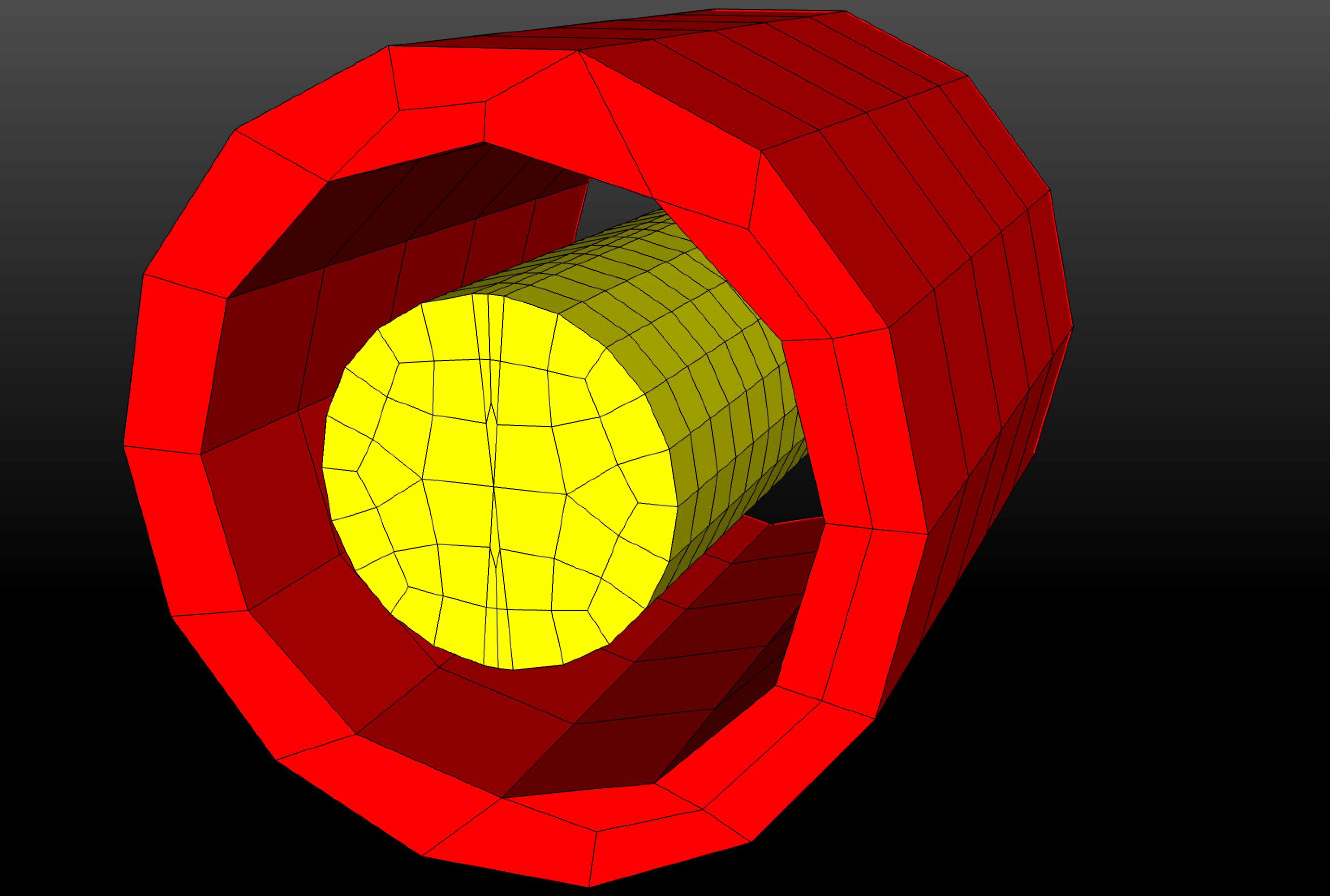(a) Initial position.

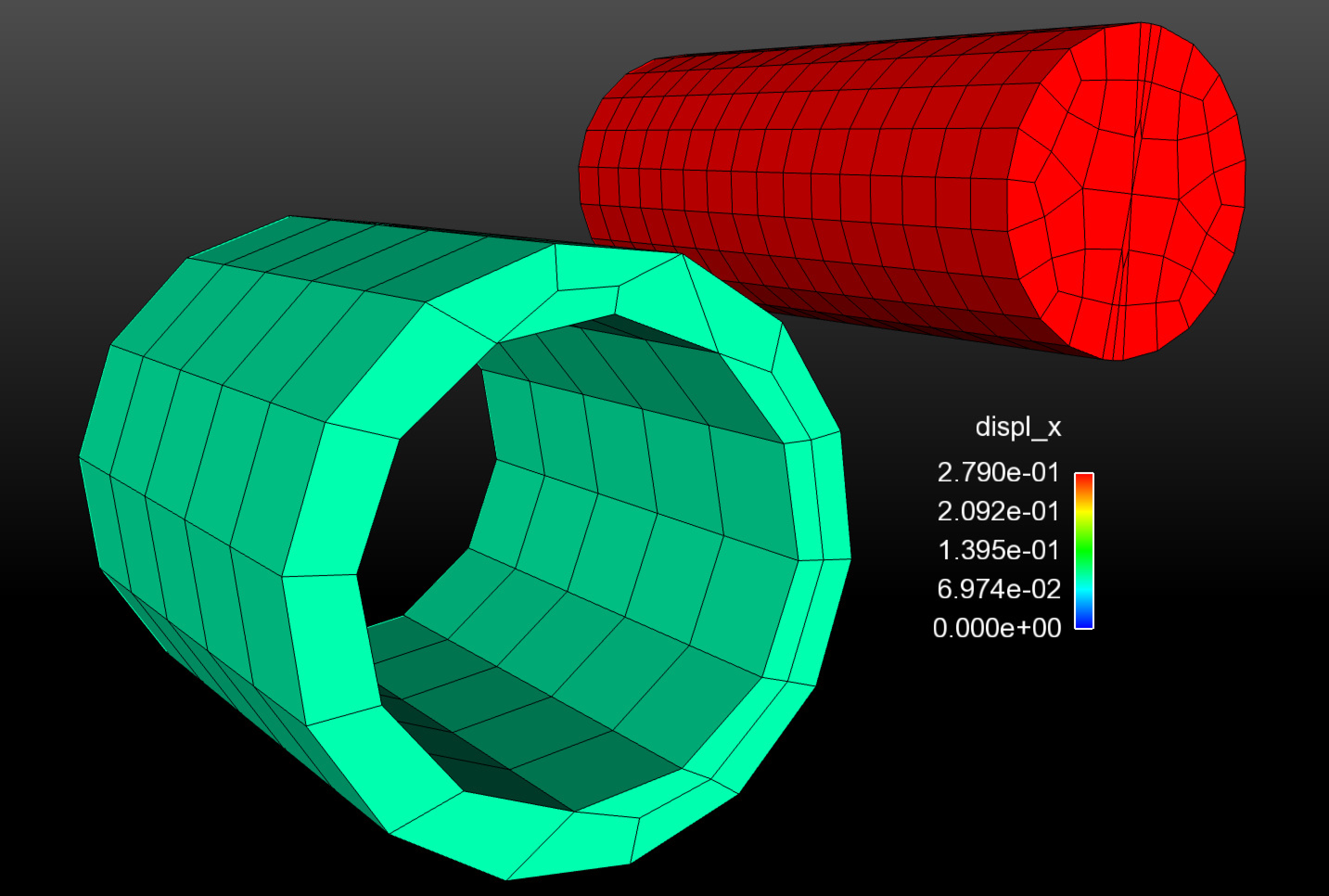(b) Final position.

Fig. 7.15 RBE3 test positions.

7.16.12. Bolt Preloading

A capability for bolt preloading exists to help streamline the definition of a very specific, but common, operation. Preloading is achieved through the strategic application of artificial strain to a specified element block. The preload target value is approached by incorporating a preload controller/solver that monitors a user-defined global output variable. The bolt preloading function makes heavy use of a production-level preloading subroutine, but with some further enhancements to improve usability and efficiency.

The available bolt preloading command syntax is as follows:

BEGIN PRELOAD
  #
  # REQUIRED: PRELOAD DEFINITIONS
  #
  PRELOAD BOLT <string>block_name1 TO TARGET USER {STRESS|FORCE} <string>global_target_var1
      = <real>target_value1 [IN DIRECTION <string>dir_name]
  PRELOAD BOLT <string>block_name2 TO TARGET USER {STRESS|FORCE} <string>global_target_var2
      = <real>target_value2 [IN DIRECTION <string>dir_name]
  ...
  PRELOAD BOLT <string>block_nameN TO TARGET USER {STRESS|FORCE} <string>global_target_varN
      = <real>target_valueN [IN DIRECTION <string>dir_name]
  (preload commands may be repeated multiple times)

  PRELOAD BOLT <string>block_name TO TARGET {AVERAGE|MAX} VON MISES
      = <real>target_valueN [IN DIRECTION <string>dir_name]
  PRELOAD BOLT <string>block_name TO TARGET INTERNAL FORCE
      = <real>target_valueN [IN DIRECTION <string>dir_name]
  #
  # OPTIONAL: PRELOAD SOLVER \& OTHER SETTINGS
  #
  EXPLICIT CONTROL ALGORITHM = INCREMENTAL|PID(INCREMENTAL)
  ITERATION TIME = <real>iter_time
  SOLVER ADAPTIVITY = ON|OFF(OFF)
  COMPUTE INTERNAL REACTION OUTPUTS = ON|OFF(OFF)
  SEPARATE COMPONENTS = ON|OFF(ON)

  #
  # OPTIONAL: ACTIVE PERIOD SETTINGS
  #
  ACTIVE PERIODS = <string list>period_names
  INACTIVE PERIODS = <string list>period_names
END

Bolt preloading in SIERRA can be achieved in a multitude of ways. The preload functionality described herein is offered as one specific method in which bolt preload may be achieved. Although the BEGIN PRELOAD command block will simply apply artificial strain as directed, users are recommended to adopt a bolted-joint geometry creation approach that mirrors what is depicted in Fig. 7.16. Specifically, the mesh entities the user wishes to preload (the shank, in this example) should be in a separate element block. The reason for this is two-fold: first, the preload operation is generally more physically appropriate and successful when other portions (bolt head, threads) are not included in the preload algorithm, and second, the target preload variable (e.g., normal force, maximum von Mises) must be computed on only the block of interest. Geometry definitions that significantly depart from this recommendation may not work as desired.

Users may place multiple bolts into a single block if desired. This is advantageous when there are multiple bolts of identical geometry and target preload criteria. When multiple bolts exist in a single block, they will be individually preloaded according to the specified target criteria. Bolts needing different preload target criteria must be placed into separate exodus blocks.

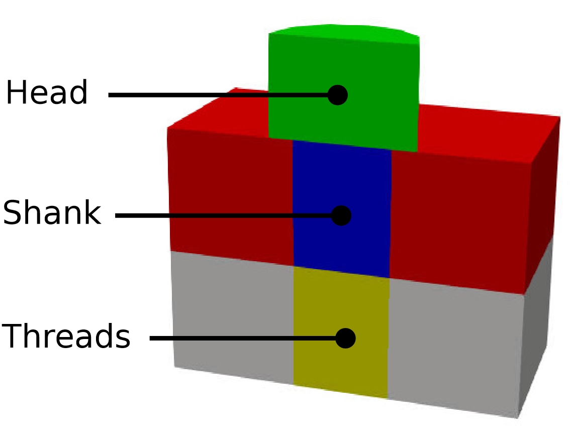
Fig. 7.16 Anatomy of a typical preloaded bolted joint. Users are recommended to place the portion of the bolt shank to be preloaded in a separate element block.

Preload solution type: implicit and explicit The preload capability supports both implicit and explicit analyses. In either case, preload is achieved through the incremental application of artificial strain. Different incrementation strategies are used for implicit and explicit analyses to accomodate the fundamental differences of these solution types.

In explicit, the preload capability is constrained by the time period during which users allow preloading to take place. As preloading is still a dynamic event when applied as part of an explicit dynamics solution, users must take care to provide sufficient time for bolt preloading to take place. For many analyses, a time period in the range of 1ms to 10ms is sufficient, but the exact time period needed will vary and may require some experimentation. A strain incrementation control strategy is used to adjust the amount of strain needed to reach a desired level of preload. Two control algorithms are available: an incremental approach (INCREMENTAL) and proportional-integral-derivative control approach (PID). Either of these explicit control algorithms is selectable via the EXPLICIT CONTROL ALGORITHM line command. Figure Fig. 7.17 illustrates the differences between these algorithms.

The INCREMENTAL control strategy is based on a preloading subroutine and has was the only control algorithm available. This control strategy increments strain using a ramp-and-hold approach. Strain is incremented using a cosine ramp by some small amount and then held constant for a period of time to allow for noise to damp out. This incrementation is repeated approximately 20x (adjustable via ITERATION TIME option) until the target preload is reached. Strain inccrements are carefully reduced as the preload target is neared to prevent overshooting the target and inducing irreversible plastic strains.

The PID control algorithm using a traditional proportional-integral-derivative control system to adjust the strain until the target is reached. An error term is computed as the difference between the desired preload and the current preload. The gain coefficients for the PID controller were selected to provide a good balance between efficiency and robustness.

The PID control strategy was added to address shortcomings of the INCREMENTAL approach when preloading bolts with large gaps. It is typically necessary to first apply enough strain to close the gap before a target preload can be reached due to the additional compliance added to the joint by a large gap. The incremental approach may not apply enough strain to close the gap, and thus may fail to reach a target preload. Although the INITIAL GUESS option can be used to manually adjust the strain size, this quickly becomes intractable. In contrast, the PID algorithm dynamically adjusts the necessary strain increment based on the current state of the model. As a result, the PID control strategy may reach the target preload faster than the INCREMENTAL approach. However, the PID control algorithm may go unstable and invert elements if the system being preloaded is particularly noisy whereas the INCREMENTAL approach has a long history and tends to work quite well even in “noisy” models. Note that the PID control algorithm does not use the ITERATION TIME and SOLVER ADAPTIVITY line commands; values provided for these options will have no effect.

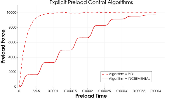
Fig. 7.17 There are two different explicit preload control algorithms available: PID and INCREMENTAL.

In implicit, the time period selection for preloading is unimportant; however, the number of time steps is relevant. For many analyses, five to ten time steps is sufficient, but the necessary number of steps will vary and may require some experimentation. In addition, rigid body modes should not be present in implicit analyses. The implicit preload control algorithm differs from explicit control algorithms in that larger time steps are used, and solutions should be quasi-static or nearly quasi-static (if implicit dynamics is enabled). Furthermore, solutions are often approximately linear. Thus, the strain required to achieve a preload target can be determined via extrapolation. The implicit preload algorithm iteratively extrapolates the required strain to reach the target preload.

A dissipation mechanism is recommended to assist with achieving a quasi-static preload state in explicit. The VELOCITY DAMPING line command in a VISCOUS DAMPING command block may be used for this purpose. An appropriate value may be in the range of 0.0001 to 0.005, although smaller or larger values may be needed and some experimentation will be necessary. The damping may be selectively disabled by using the ACTIVE PERIODS or INACTIVE PERIODS after the preloading time period has ended if desired.

Inside the BEGIN PRELOAD command block, users may specify the PRELOAD BOLT line command any number of times.

#
# REQUIRED: PRELOAD DEFINITIONS
#
PRELOAD BOLT <string>block_name TO TARGET USER {STRESS|FORCE} <string>global_target_var
    = <real>target_value [IN DIRECTION <string>dir_name]
PRELOAD BOLT <string>block_name TO TARGET {AVERAGE|MAX} VON MISES
    = <real>target_valueN [IN DIRECTION <string>dir_name]
PRELOAD BOLT <string>block_name TO TARGET INTERNAL FORCE
    = <real>target_valueN [IN DIRECTION <string>dir_name]

The PRELOAD BOLT line command will cause unidirectional artificial strain to be applied to block_name (which may also be an assembly) in the specified direction. Assemblies may contain blocks, or assemblies of these.

Establishing a preload direction The preload direction may be explicitly specified using a direction defined at the SIERRA scope. Predefined directions GLOBAL_(X|Y|Z) are also available without additional definition at the SIERRA scope for convenience. Alternatively, if the preload direction is omitted a default direction will be automatically computed. For solid elements, the automatically-computed direction is determined from the geometry of block_name or assembly_name as the principal axis corresponding to the minimum (or maximum) eigenvalue of the moment of inertia tensor. For the common case of a relatively-long cylindrical shaft or relatively thin disk, this is the desired axial direction. However, results should be verified when using automatic directions (in results output, and also in the log file where an initialization summary table is available). For beam elements, the local x-direction is the only meaningful preload direction and is automatically used regardless of geometry.

Setting preload target (built-in) Preload commands must specify the desired method of preload, generally as a global quantity. Three common use-cases are available as “presets” and can be used without any further user input: TO TARGET MAX VON MISES, TO TARGET AVERAGE VON MISES, and TO TARGET INTERNAL FORCE. These preload commands will cause the preload algorithm to iterate until the von Mises stress or the net internal axial force reach the specified target values.

The TARGET MAX VON MISES command causes the preload algorithm to seek an artificial strain for which the maximum element von Mises (in the specified preload block) equals the specified target value. In the case of multiple integration point elements, the target is reached when any single integration point reaches the maximum value. Beware that stress concentrations in the preloaded entity are likely, and may result in a net preload that is less than intended. Therefore, this preset should be used with appropriate care to avoid unintended behavior. Unintended behavior may possibly be avoided by preloading a section of a bolt shank that does not include elements adjacent to the bolt head.

The TARGET AVERAGE VON MISES command causes the preload algorithm to seek an artificial strain for which the average von Mises value equals the specified target value. The average is an arithmetic mean of the element von Mises variable at all integration points of the preloaded entity. This may provide a more accurate measure of stress in a bolt shank which contains stress concentrations. However, care must be taken to ensure no extraneous elements are included in the preload entity to avoid unintended behavior. For example, failure to separate the bolt head from the shank may include elements with near-zero von Mises stress in the average calculation and cause a larger preload than intended. Furthermore, it is possible that stress concentrations may cause localized yielding to occur in the presence of plasticity constitutive models despite the average value remaining below yield.

The TARGET INTERNAL FORCE command causes the preload algorithm to seek an artificial strain for which the net reaction force in the direction of preloading equals the specified target value. The reaction force is calculated by identifying a plane and normal direction which splits the preloaded entity at its centroid. The net reaction force is calculated by summing the internal element forces into a single force representing the net tensile force in the preloaded entity. This calculation requires at least two “layers” of elements such that there are elements on both the top and bottom of the cutting plane.

Setting preload target (user-defined) Preloading to reach other target quantities is also supported, but requires a user-defined global variable global_target_var to be specified in the input deck. This must be done via a USER OUTPUT command block which computes some global quantity of interest (such as average von Mises stress) over the block with name block_name (or assembly). The line command COMPUTE AT EVERY STEP must be specified as part of the user output block. Depending on the nature of the desired target variable, it may also be necessary to manually provide an initial guess. The syntax TO TARGET USER {STRESS|FORCE} specifies that the target global variable is a stress-like quantity or a force-like quantity, respectively, so that the preload algorithm can properly estimate the required strain needed to reach the target value.

Active preload period During the time period in which the PRELOAD command block is active, a preload controller/solver will incrementally apply an artificial strain until a target value target_value is reached, or until the active time period (or analysis) terminates. At the end of the preload operation, a table containing diagnostic information will be output to the log file for reference. Data included in the table assists with knowing the final preload in each bolt, the required strain to reach that preload (may be used in subsequent analyses directly, without preload iterations), and a quick go/no-go indicator for if all preload targets were reached.

Preloading multiple bolts The PRELOAD BOLT line command may be repeated within the BEGIN PRELOAD command block any number of times. If a specified block or assembly contains multiple representations of a bolt (physically disconnected components), the preload command line will apply to each bolt individually, such that each separated body was preloaded to the target value. The direction may be determined automatically so that bolts need not be aligned.

A separate preload controller/solver will be created for each line command. Currently, preloading in explicit dynamics behaves nearly identically to the aupst_preload_solver subroutine. This subroutine is used to drive preloads to their target values by slowly ramping up unidirectional artificial strain.

Tabular preload summaries A tabular summary will be output at the end of the preload time period or analysis, whichever comes first. The tabular summary will list the block name being preloaded, the percentage and value of preload achieved relative to the target, and the amount of artificial strain applied at the termination of the preloading operation. These values are offered for reference or may be used to directly apply artificial strain to a specific value in future repeat analyses. For example, an explicit preloading analysis may be used to determine the required artificial strain to achieve a desired preload. The results of that analysis may be used in an implicit analysis to quasi-statically apply preload over just a few time steps since the required value is known a priori.

Variables for monitoring preload:

A nodal variable sm_preload_internal_reaction_plane will be created to visualize the cutting plane that internal reaction is using in the preload.

A set of output variables are also created for each preload line command. A global variable named sm_preload_strain_<block_name> will be created for each PRELOAD BOLT line command. For example, the preload line command given as:

PRELOAD BOLT bolt1_shank TO TARGET max_von_mises_bolt1 = 8000
   IN DIRECTION GLOBAL_X

would generate a global variable named sm_preload_strain_bolt1_shank that could be monitored as necessary. The preload magnitude could be monitored using the user-defined output variable max_von_mises_bolt1. If multiple bolts exist in the same block, a suffix _Component<num> is added to the global variable name so that target values may be monitored separately. For example, if bolt1_shank contained two bolts, their strain values would be found in variables sm_preload_strain_bolt1_shank_Component0 and sm_preload_strain_bolt1_shank_Component1. An element variable named sm_preload_strain is generated which may be used to visualize the amount of strain applied to each bolt.

Optional commands Although the default options are generally designed to achieve target preload without further intervention, several optional commands are available to influence the preload algorithm.

#
# OPTIONAL: PRELOAD SOLVER & OTHER SETTINGS
#
EXPLICIT CONTROL ALGORITHM = INCREMENTAL|PID(INCREMENTAL)
ITERATION TIME = <real>iter_time
SOLVER ADAPTIVITY = ON|OFF(OFF)
COMPUTE INTERNAL REACTION OUTPUTS = ON|OFF(OFF)
SEPARATE COMPONENTS = ON|OFF(ON)

The preload algorithm incrementally applies artificial strain over a time period given by iter_time. By default, this value is automatically determined by the duration of the allotted preload period such that 20 strain incrementation cycles will occur (relevant for the default INCREMENTAL control strategy only). The user may override this default value by specifying a value for ITERATION TIME. The strain incrementation over each iteration is automatically determined based on preload geometry, material properties, and target value. The ITERATION TIME option does not affect the PID control algorithm.

The SOLVER ADAPTIVITY line command may be used to enhance the INCREMENTAL preload subroutine. By monitoring the preload solution for overshoot and convergence, the time period over which strain increments are applied, or the magnitude of a strain increment, may be adaptively changed to increase the solution efficiency. For example, if a very small overshoot is detected the time increment could be cut back such that a target preload is achieved more quickly. The solver adaptivity options are currently limited (for example, there is no growth when overshoot is detected) so this option is disabled by default. However, users may experiment with the option as desired. Users are advised to only enable this command for troubleshooting a very specific issue in which the automatically determined strain increment is not sufficient to reach target preload. Generally, selecting the PID control algorithm may be a better solution and may address the same sort of issues that (e.g. large gaps).

The COMPUTE INTERNAL REACTION OUTPUTS line command will optionally compute global output variables named sm_preload_axial_force_<block_name> whose values are the net axial force in the bolt. The net axial force is computed using the same method as the COMPUTE ... AS INTERNAL REACTION line command offers in a USER OUTPUT command block (see Section 9.4.2). This output is disabled by default to avoid unnecessary calculation when it is not needed. This output is provided as a convenience for monitoring preload over the entire analysis. If multiple bolts exist in the same block, a suffix _Component<num> is added to the global variable name.

Warning

Note that for the sm_preload_axial_force_<block_name> variables to be properly computed, there must be at least two solid elements along the axial direction of the preloaded bolt/entity or else the reported force will be zero. Beam elements do not suffer this limitation.

The preload command line will typically apply to each bolt in a block or assembly individually. The SEPARATE COMPONENTS line command may be used to disable this feature; however, this is not suggested for most applications. In particular, this feature may only be disabled if all bolts within each block or assembly are to be loaded in the same direction.

The BEGIN PRELOAD may also be restricted to specific time periods via the usual ACTIVE PERIODS and INACTIVE PERIODS line commands as described in Section 2.6. Although the use of these commands is optional, users are advised to provide only a single active period for preloading. The first time period in which preloading is active will determine the duration over which strain increments are applied, which may influence the amount of noise and overshoot introduced in each preload solver iteration. The preload solver will continue being active into subsequent time periods as specified. Thus, if one wishes to cause the preload solver to iterate more than the default iteration time allows for, a second time period could be added. In some circumstances, this approach may allow for further dynamic relaxation and reduction of noise in the system.

#
# OPTIONAL: ACTIVE PERIOD SETTINGS
#
ACTIVE PERIODS = <string list>period_names
INACTIVE PERIODS = <string list>period_names

There are several recommendations and limitations that users must be aware of when using the bolt preloading command block.

• Bolts of solid element should be constructed nominally as depicted in Fig. 7.16. The objective is to isolate the bolt shank from the rest of the body so that it can be preloaded separate from the head or threaded portion of the bolt shank. Beam elements should be straight and should not specify a direction.

• The COMPUTE AT EVERY STEP option must be specified in the user-defined target variable to ensure accurate and up-to-date values are available for the preload controller.

• The use of a single time period is recommended. The preload solver option uses the starting and stopping times of the first preload time period to determine the time period over which preload is incremented when not specified explicitly by the ITERATION TIME command.

• A sufficiently long time period, relative to the physical system under consideration, must be specified for the preload to occur. This duration is often on the order of 1 ms to 10 ms.

• Some form of viscous damping is recommended for explicit analyses.

---

[1] (1,2,3)

K.H. Brown, J.R. Koteras, D.B. Longcope, and T.L. Warren. CavityExpansion: a library for cavity expansion algorithms, version 1.0. Technical Report SAND2003-1048, Sandia National Laboratories, Albuquerque, NM, April, 2003. URL: http://infoserve.sandia.gov/sand_doc/2003/031048.pdf.

[2]

J. Lysmer and R.L. Kuhlmeyer. Finite dynamic model for infinite media. In Proceedings of the American Society of Civil Engineers, 859–877. 1979.