13. Nonlinear Equation Solving

13.1. Introduction

This chapter discusses non-linear equation solving methods, specifically the use of iterative algorithms for problems in solid mechanics. Although some of this work has taken place over many years at Sandia National Labs and elsewhere, recent efforts have significantly added to the functionality and robustness of these algorithms. This chapter primarily documents these recent efforts. Some historical development is covered for context and completeness, hopefully showing a complete picture of the current status of iterative solution algorithms for nonlinear solid mechanics in Sierra/SolidMechanics.

Iterative algorithms have seen somewhat of a resurgent interest, possibly due to the advancement of parallel computing platforms. Increases in computational speed and available memory have raised expectations on model fidelity and problem size. Increased problem size has sparked interest in iterative solvers because the direct solution strategy becomes increasingly inefficient as problem size grows. A traditional implicit global solution strategy is typically based on Newton’s method, generating fully coupled linearized equations that are often solved using a direct method. In many applications in solid mechanics this procedure poses no particular problem for modern computing platforms with sufficient memory. However, for large three-dimensional models of interest, the cost of direct equation solving becomes prohibitive on any computer, except for the largest supercomputers. This motivates the use of iterative solution strategies that do not require the direct solution of linearized global equations.

Application of purely iterative solvers to the broad, general area of nonlinear finite element solid mechanics problems has seen only modest success. Certain classes of problems have remained notoriously difficult to solve. Examples of these include problems that are strongly geometrically nonlinear, problems with nearly incompressible material response, and problems with frictional sliding. Thus, much of this chapter is devoted to examining and discussing an implementation of a multi-level solution strategy, where the nonlinear iterative solver is asked to solve simplified model problems from which the real solution to these difficult problems is accumulated. This strategy has greatly contributed to the functionality and robustness of the nonlinear iterative solver.

13.2. The Residual

(13.1)\[\mathbf{r} \left( \mathbf{d}_{n+1} \right) = \mathbf{F}^{\mathrm{ext}} \left( \mathbf{d}_{n+1}\right) - \mathbf{F}^{\mathrm{int}} \left( \mathbf{d}_{n+1} \right) = \mathbf{0}\]

and the implicit dynamics problem using the trapezoidal time integration rule, (12.46), is written as

(13.2)\[\mathbf{r} ( \mathbf{d}_{n+1}) = \left[ \mathbf{F}^{\mathrm{ext}}(\mathbf{d}_{n+1}) + \mathbf{M} \left( \mathbf{a}_n + \Delta t ~ \mathbf{v}_n + \frac{4}{\Delta t^2} \mathbf{d}_n \right) - \left( \frac{4}{\Delta t^2} \mathbf{M} \mathbf{d}_{n+1} + \mathbf{F}^{\mathrm{int}}(\mathbf{d}_{n+1}) \right) \right] = \mathbf{0} .\]

In either case, the equation to be solved takes the form

(13.3)\[\mathbf{r} \left( \mathbf{d}_{n+1} \right) = \mathbf{0} ,\]

where the residual \(\mathbf{r} \left( \mathbf{d}_{n+1} \right)\) is, in general, a nonlinear function of the solution vector \(\mathbf{d}_{n+1}\). This form allows us to consider the topic of nonlinear equation solving in its most general form, with the introduction of iterations, \(j=0,1,2, ...\), as

(13.4)\[\mathbf{r} \left( (\mathbf{d}_{n+1})_j\right) = \mathbf{0} ,\]

or simply

(13.5)\[\mathbf{r}_j = \mathbf{r} \left( \mathbf{d}_j \right) = \mathbf{0}.\]

For implicit dynamic Sierra/SM simulations, each load step from time \(n\) to \(n+1\) requires a new nonlinear solve with sub-iterations \(j=0,1,2,...\). Here we have omitted the references to the load step, yet it is understood that, e.g., \(\mathbf{d}_j\) is at \(n+1\).

We can rewrite (13.1) and (13.2) as

(13.6)\[\mathbf{r}_j = \mathbf{F}^{\mathrm{ext}}_j - \mathbf{F}^{\mathrm{int}}_j = \mathbf{0}\]

and

(13.7)\[\mathbf{r}_j = \mathbf{F}^{\mathrm{ext}}_j - \frac{4}{\Delta t^2} \mathbf{M} \mathbf{d}_j - \mathbf{F}^{\mathrm{int}}_j + \tilde{\mathbf{F}} = \mathbf{0}\]

where \(\mathbf{F}^{\mathrm{int}}_j = \mathbf{F}^{\mathrm{int}} \left( \mathbf{d}_j \right) = \mathbf{F}^{\mathrm{int}} \left( (\mathbf{d}_{n+1})_j \right)\) and \(\tilde{\mathbf{F}}\) is the constant portion of the residual, defined as

\[\tilde{\mathbf{F}} = \mathbf{M} \left( \mathbf{a}_n + \Delta t ~ \mathbf{v}_n + \frac{4}{\Delta t^2} \mathbf{d}_n \right).\]

The task for any nonlinear equation solution technique is to improve the iterate (or guess) for the solution vector \(\mathbf{d}_j\) such that the residual \(\mathbf{r}_{j}\) is close enough to \(\mathbf{0}\). How that is done depends on the method employed.

Fig. 13.1 depicts a generalized nonlinear loadstep solution with solution iterates \(j=0,1,2, ..., j^*\), where the iterates converge when \(\left\lVert\mathbf{r}_{j^*}\right\rVert \approx 0\) at iteration \(j^*\).

In (a) of Fig. 13.1, the solution starts with iterate \(\mathbf{d}_0\) taken as the solution of the prior load step from \(n-1\) to \(n\). (Note that the zero iterate is not always taken to be the prior solution. See Section 13.6.4 on predictors for more details.) Iterate \(\mathbf{d}_0\) results in a residual of \(\mathbf{r}_0\), which then informs the next iterate \(\mathbf{d}_1\) such that \(\left\lVert\mathbf{r}_1\right\rVert < \left\lVert\mathbf{r}_0\right\rVert\). For details on how \(\mathbf{d}_1\) is formed, see the following Sections Section 13.3 through Section 13.8. In (b) and (c) this procedure from iteration \(j\) to \(j+1\) is depicted, and in (d) the solution procedure has converged at iteration \(j^*\) with iterate \(\mathbf{d}_{j^*}\). The load step from \(n\) to \(n+1\) is then solved, and the solution procedure for the next load step from \(n+1\) to \(n+2\) starts over in (a).

Fig. 13.1 Graphical depiction of nonlinear iterations.

13.3. Gradient Property of the Residual

The residual has the very important property that it points in the steepest descent or gradient direction of the function \(f\):

(13.8)\[f \left( \mathbf{d}_j \right) = \frac{1}{2} \left( \mathbf{d}_j - \mathbf{d}^{*} \right) ^T \mathbf{r} (\mathbf{d}_j),\]

which is the energy error of the residual. Solving for \(\mathbf{d}_j = \mathbf{d}^{*}\) is equivalent to minimizing the energy error of the residual, \(f \left( \mathbf{d}_j \right)\).

The importance of this property can not be overemphasized. Any iterative solver makes use of it in some way or another. Even though the solution \(\mathbf{d}^{*}\) is not known, a non-zero residual points the way to improving the guess. Mathematically, our nonlinear solid mechanics problem looks like a minimization problem discussed at length in the optimization literature, see e.g. [[1]]. It is from this viewpoint that the remainder of the nonlinear solution methods will be discussed. The concept of the energy error of the residual reveals important physical insights into how iterative algorithms are expected to perform on particular classes of problems.

An example of the energy error of the residual providing physical insight into a problem is demonstrated in Fig. 13.2.

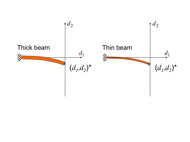
Fig. 13.2 Energy error example: two beams with large and small \(x\)-sectional moments of inertia.

Two beams, one thick and one thin, are subjected to a uniform pressure load causing a downward deflection to the equilibrium point \((d_1,d_2)\) indicated by the blue dot. If we think of modes of deformation rather than the nodal degrees of freedom \((d_1 ,d_2 )\), two modes of deformation come to mind: a bending mode and an axial mode.

Fig. 13.3 Energy error example: modes of deformation for two beams.

For the thick beam in Fig. 13.3, the red dashed line is the locus of points \((d_1,d_2)\) that induce only bending stresses in the beam and is therefore called a bending mode. In contrast, the blue dashed line is the locus of points \((d_1,d_2)\) that induce only axial stresses in the beam and is therefore called an axial mode. These bending and axial modes are characterized by the eigenvectors \(q_b\) and \(q_a\), respectively.

Eigenvectors are typically written as linear combinations of the nodal degrees of freedom. The bending modes, for example, can be written as \(q_b = a_1 d_1 + a_2 d_2\). However, since we are dealing with a nonlinear problem in our simple example (and in general), the coefficients \(a_1\) and \(a_2\) vary with the deformation of the beam - which is precisely why the dashed red line is curved. The energy error contours can thus be displayed, as shown in Fig. 13.4. Any displacement away from the equilibrium point \((d_1,d_2)^{*}\) produces a nonzero residual and consequently requires work.

Fig. 13.4 Energy error example: energy error contours for two beams.

Now we compare moving the tip of the beam along the red dashed line, which invokes a bending mode of deformation of the beam versus moving the tip along the blue dashed line, which invokes an axial mode of deformation. The larger modal stiffness (eigenvalue) corresponding to the axial mode induces a greater energy penalty for a given amount of displacement compared to the bending mode. This produces the stretched energy contours shown. Since the ratio of stiffness between the axial and bending modes is much larger for the thin beam than the thick beam, the stretching of the energy error contours is more pronounced for the thin beam. Mathematically, these contours are a graphical representation of the gradient of the residual, \(\nabla \mathbf{r}(\mathbf{d})\).

The beam example is chosen for its simplicity, however it also poses a non-trivial nonlinear problem. Experience has shown that the thinner the beam becomes the more difficult it is to solve. In fact, convergence investigations reveal that it is the ratio of maximum to minimum eigenvalue of \(\nabla \mathbf{r}(\mathbf{d})\) that is critical to the performance of iterative methods.

13.4. Newton’s Method for Solving Nonlinear Equations

In this context, the idea embodied in classical Newton’s method is simple. Substituting the nonlinear residual \(\mathbf{r}(\mathbf{d}_j)\) with the local tangent approximation \(\mathbf{y}(\mathbf{d})\) gives

(13.9)\[\mathbf{y} (\mathbf{d}) = \mathbf{r}(\mathbf{d}_j) + \nabla \mathbf{r} (\mathbf{d}_j) (\mathbf{d}-\mathbf{d}_j),\]

which is linear in the vector of unknowns \((\mathbf{d})\). Solving (13.9) (solving for \(\mathbf{y}(\mathbf{d}) = \mathbf{y}(\mathbf{d}_{j+1}) = \mathbf{0}\)) gives the iterative update for Newton’s method,

(13.10)\[\mathbf{d}_{j+1} = \mathbf{d}_j - \nabla \mathbf{r}^{-1} (\mathbf{d}_j) \mathbf{r} (\mathbf{d}_j).\]

The structural mechanics community commonly refers to the tangent stiffness matrix in the context of geometrically nonlinear problems. Based on (13.9), the tangent stiffness matrix arises from the tangent approximation of \(f(\mathbf{d}_j)\):

(13.11)\[\mathbf{K}_T = \nabla \mathbf{r} (\mathbf{d}_j).\]

Then (13.10) can be written as

(13.12)\[\mathbf{d}_{j+1} = \mathbf{d}_j - \left[ \mathbf{K}_T \right]^{-1} \mathbf{r} (\mathbf{d}_j) ,\]

the solution of which requires the inverse of \(\mathbf{K}_T\).

A conceptual view of Newton’s method applied to our two beam example is shown in Fig. 13.5.

Fig. 13.5 Energy error example: Newton’s method applied to two beams.

Newton’s method is generally considered to be the most robust of the nonlinear equation solution techniques, albeit at the cost of generating the tangent stiffness matrix (13.11) and solving the linear system of equations with \(n_{dof}\) unknowns:

(13.13)\[\left[ \mathbf{K}_T \right] \left( \mathbf{d}_{j+1} - \mathbf{d}_j \right) = - \mathbf{r} (\mathbf{d}_j).\]

There are a number of linear equation solution techniques available, and Sierra/SolidMechanicshas the ability to apply a linear equation solution approach available in the FETI library (discussed briefly in section Section 13.7).

As mentioned, Newton’s method relies on computing the tangent stiffness matrix which, by examination of (13.14), requires the partial derivatives (with respect to the unknowns) of the external and internal force vector,

(13.14)\[\mathbf{K}_T = \frac{\partial}{\partial \mathbf{d}} \left[ \mathbf{F}^{\mathrm{ext}}_j - \mathbf{F}^{\mathrm{int}}_j \right].\]

In practice, for all but the simplest of material models, the exact tangent cannot be computed. Thus Sierra/SolidMechanics computes a secant approximation with the property

(13.15)\[\mathbf{K}_{\tilde{T}} \cdot \left( \delta \mathbf{d} \right) = \mathbf{r} (\mathbf{d}_j + \delta \mathbf{d}) - \mathbf{r} (\mathbf{d}_{j})\]

by simply probing the nonlinear system via perturbations \(\delta \mathbf{d}\). In (13.15), the notation \(\mathbf{K}_{\tilde{T}}\) is used to indicate that the probed tangent is an approximation of the exact tangent.

13.5. Steepest Descent Method

As mentioned in section Section 13.3, the steepest descent iteration takes steps in the direction of the gradient of the energy error of the residual. On its own, it would not be considered a viable solver for solid mechanics because of its general lack of performance compared to Newton-based methods. However, there are algorithmic elements of this method that are conceptually important for understanding nonlinear iterative solver such as the method of conjugate gradients, and in fact are used in their construction.

The idea behind the steepest descent method is to construct a sequence of search directions, \(\mathbf{s}_j\),

(13.16)\[\mathbf{s}_j = \mathbf{M}^{-1} \mathbf{g}_j = -\mathbf{M}^{-1} \mathbf{r} (\mathbf{d}_j),\]

in which the energy decreases, thus producing a new guess of the solution vector

(13.17)\[\mathbf{d}_{j+1} = \mathbf{d}_j + \alpha \mathbf{s}_j.\]

The minimization is accomplished by taking a step of length \(\alpha\) along \(\mathbf{s}_j\), where \(\alpha\) is called the line search parameter:

(13.18)\[\frac{\mathrm{d}}{\mathrm{d} \alpha} f(\mathbf{d}_j + \alpha \mathbf{s}_j ) \approx \left[ \mathbf{r} (\mathbf{d}_j ) \right] ^T \mathbf{s}_j + \alpha \left[ \mathbf{r} (\mathbf{d}_j + \mathbf{s}_j ) - \mathbf{r} (\mathbf{d}_j ) \right] ^T \mathbf{s}_j = 0 ,\]

which, after simplification, gives

(13.19)\[\alpha = \frac{ \left[ \mathbf{r} (\mathbf{d}_j ) \right] ^T \mathbf{s}_j } { \left[ \mathbf{r} (\mathbf{d}_j + \mathbf{s}_j) - \mathbf{r} (\mathbf{d}_j ) \right] ^T \mathbf{s}_j }.\]

The preconditioner matrix \(\mathbf{M}\) is included in (13.16) to accelerate the convergence rate of the steepest descent method. Note that in this case \(\mathbf{M}\) is not meant to be the mass matrix.

Fig. 13.6 through Fig. 13.8 all show high aspect ratio ellipses. It turns out that the ideal preconditioner would transform the ellipses to circles; this, in turn, would be \(\mathbf{M} =\mathbf{K}_T\). As expected, the ideal steepest descent method is Newton’s method. However, the steepest descent framework gives us a way to use approximations of \(\mathbf{K}_{T}\).

A conceptual view of the steepest descent method applied to our two beam example is shown in Fig. 13.6. As indicated in the figure, the thinner beam would require more steepest descent iterations to obtain convergence compared to the thicker beam.

Fig. 13.6 Energy error example: Steepest descent method applied to two beams.

It is instructive to consider whether or not the large number of iterations are due to the nonlinearities in this model problem. For this purpose, we construct the two beam model problem in linearized form. Fig. 13.7 shows the first iteration of the steepest descent method for the linearized problem. The immediate difference seen between the linearized version and the nonlinear problem is in the elliptic form of the energy error contours. However, the contours are still stretched reflecting the relative modal stiffness of the axial and bending modes. Thus, from the same starting point, \(d_1 = d_2=0\), the initial search direction is composed of different amounts of \(d_1\) and \(d_2\). This is also apparent in all subsequent iterations. Fig. 13.8 shows the completed iterations for both thick and thin beams.

Fig. 13.7 Energy error example: First two iterations of the steepest descent method applied to linearized version of the two beam problem.

Fig. 13.8 Energy error example: Steepest descent method applied to linearized version of the two beam problem.

Even for the linearized problem, there is a large difference in the number of iterations required for the steepest descent method to converge for the two beams. We can see this because the slope of the search directions is smaller for the thin beam. Therefore, each iteration makes less progress to the solution.

In general, the convergence rate of the steepest descent method is directly related to the spread of the eigenvalues in the problem. In our conceptual beam example, the ratio \(\lambda_{\mathrm{max}} / \lambda_{\mathrm{min}} = \lambda_a / \lambda_b\) (often called the condition number) is larger for the thin beam. It can be shown that in the worst case, the steepest descent iterations reduce the energy error of the residual according to

(13.20)\[f( \mathbf{d}_{j+1}) = \left( \frac {\lambda_{\mathrm{max}} / \lambda_{\mathrm{min}} - 1} {\lambda_{\mathrm{max}} / \lambda_{\mathrm{min}} + 1} \right)^2 f( \mathbf{d}_j ) .\]

13.6. Method of Conjugate Gradients

With the foundation provided by the steepest descent method, application of a conjugate gradient algorithm to (13.6) or (13.7) follows in a straightforward manner. Like the steepest descent method, the important feature the conjugate gradient (or CG) algorithm is that it only needs to compute the nodal residual vectors element by element, and as a result, does not need the large amount of storage required for Newton’s method.

The method of conjugate gradients is a well-developed algorithm for solving linear equations. Much of the original work can be found in the articles [[2][3][4]] and the books [[5][6]]. A convergence proof of CG with inexact line searches can be found in [[7]], and a well-presented tutorial of linear CG can be found in [[8]]. The goal here is to review the method of conjugate gradients to understand the benefits and potential difficulties encountered when applying it to the solution of the nonlinear equations in solid mechanics problems.

13.6.1. Linear CG

The CG algorithm also uses the gradient, \(\mathbf{g}_j\), to generate a sequence of search directions \(\mathbf{s}_j\) for iterations \(j=1,2,...\):

(13.21)\[\mathbf{s}_{j} = -\mathbf{M}^{-1} \mathbf{r}(\mathbf{d}_j) + \beta_j \mathbf{s}_{j-1} .\]

Note the additional (rightmost) term in (13.21) relative to the steepest descent algorithm of (13.16). The scalar \(\beta_j\) is chosen such that \(\mathbf{s}_j\) and \(\mathbf{s}_{j-1}\) are \(\mathbf{K}\)-conjugate; this property is key to the success of the CG algorithm. Vectors \(\mathbf{s}_j\) and \(\mathbf{s}_{j-1}\) are \(\mathbf{K}\)-conjugate if

(13.22)\[\mathbf{s}_{j}^T \mathbf{K} \mathbf{s}_{j-1} = 0,\]

where \(\mathbf{K}\) is the stiffness matrix. For a linear problem, \(\mathbf{K}\) is a constant positive definite matrix (assuming the internal force of (13.14) is linear). Combining (13.21) and (13.22) gives the following expression for the search direction:

(13.23)\[\mathbf{s}_{j} = \frac{\mathbf{g}_{j}^T \mathbf{K} \mathbf{s}_{j-1}} {\mathbf{s}_{j-1}^T \mathbf{K} \mathbf{s}_{j-1} }.\]

Effective progress toward the solution requires minimizing the energy error of the residual along proposed search directions. As with the steepest descent method, the line search performs this function. Minimizing the energy error of the residual along the search direction occurs where the inner product of the gradient and the search direction is zero:

(13.24)\[\begin{split}\begin{aligned} \mathbf{g}_{j}^T (\Delta \mathbf{d}_j + \alpha \mathbf{s}_j ) \mathbf{s}_j & = \left[ \Delta \mathbf{F}^{\mathrm{ext}}(t) - \mathbf{K} \cdot (\Delta \mathbf{d}_j + \alpha \mathbf{s}_j ) \right] ^T \mathbf{M}^{-1} \mathbf{s}_j \\ & = \left[ (\Delta \mathbf{F}^{\mathrm{ext}}(t) - \mathbf{K} \cdot (\Delta \mathbf{d}_j )^T - ( \mathbf{K} \cdot \alpha \mathbf{s}_j ) ^T \right] \mathbf{M}^{-1} \mathbf{s}_j \\ & = \mathbf{g}_j^T \mathbf{s}_j - \alpha_j \mathbf{s}_j^T \mathbf{K}^T \mathbf{M}^{-1} \mathbf{s}_j \\ & = 0. \end{aligned}\end{split}\]

Solving (13.24) gives an exact expression for the line search parameter \(\alpha\),

(13.25)\[\alpha_{j} = \frac{\mathbf{g}_{j}^T \mathbf{s}_j } {\mathbf{s}_{j}^T \mathbf{M}^{-1} \mathbf{K} \mathbf{s}_{j} },\]

due to the inherent symmetry of \(\mathbf{K}\).

The essential feature of the method of conjugate gradients is that once a search direction contributes to the solution, it need never be considered again. As a result, the inner product of the error \(\mathbf{e}\) changes from iteration to iteration in the following manner

(13.26)\[\begin{split}\begin{gathered} \mathbf{e}_{j+1} \mathbf{K} \mathbf{e}_{j+1} - \mathbf{e}_{j} \mathbf{K} \mathbf{e}_{j} = \\ \left[ \sum_{i=j+1}^{n-1} \delta_i \mathbf{s}_i \right]^T \mathbf{K} \left[ \sum_{i=j+1}^{n-1} \delta_i \mathbf{s}_i \right] - \left[ \delta_j \mathbf{s}_j + \sum_{i=j+1}^{n-1} \delta_i \mathbf{s}_i \right]^T \mathbf{K} \left[ \delta_j \mathbf{s}_j + \sum_{i=j+1}^{n-1} \delta_i \mathbf{s}_i \right] \\ = -\left[ \delta_j \mathbf{s}_j \right]^T \mathbf{K} \left[ \delta_j \mathbf{s}_j \right]. \end{gathered}\end{split}\]

Since \(\mathbf{K}\) is constant and positive definite, the energy error of the residual decreases monotonically as the iterations proceed. Choosing \(\beta_j\) such that the property in (13.22) holds gives the important result that the sequence of search directions \(\mathbf{s}_1 , \mathbf{s}_2, ...\) spans the solution space in at most \(n_{eq}\) iterations. Furthermore, (13.26) reveals that the search directions \(\mathbf{s}_1 , \mathbf{s}_2, ...\) reduce the error in the highest eigenvalue mode shapes first and progressively move to lower ones.

An additional important numerical property of CG is that it can tolerate some inexactness in the line search as discussed in [[9]] and still maintain its convergence properties.

Applying linear CG to our simple linearized beam model problem would generate the comparison depicted in Fig. 13.9. The fact that the linear CG algorithm precisely converges in two iterations demonstrates the significance of the orthogonalization with the previous search direction.

Fig. 13.9 A comparison of steepest descent and linear CG methods applied to the linearized beam example.

13.6.2. Nonlinear CG

For fully nonlinear problems, where the kinematics of the system are not confined to small strains, the material response is potentially nonlinear and inelastic, and the contact interactions feature potentially large relative motions between surfaces with frictional response, the residual is a function of the unknown configuration at \((n+1)\), as indicated in (13.1) and (13.2).

Nonetheless, in application of linear CG concepts, it is typical to proceed with the requirement that the new search direction satisfy

(13.27)\[\mathbf{s}_j^T ( \mathbf{g}_j - \mathbf{g}_{j-1} ) = 0.\]

A comparison of (13.27) and (13.22) reveals that \((\mathbf{g}_j - \mathbf{g}_{j-1} )\) can be interpreted to mean the instantaneous representation of \(\mathbf{K}^{NL} \mathbf{s}_{j-1}\) to the extent that the incremental solution is known and therefore, how it influences the residual.

Combining (13.21) and (13.27) gives the following result for the search direction

(13.28)\[\mathbf{s}_j = \beta_j \mathbf{s}_{j-1} - \mathbf{g}_{j} = \left( \frac{\mathbf{g}_j^T ( \mathbf{g}_j - \mathbf{g}_{j-1} ) }{\mathbf{s}_{j-1}^T ( \mathbf{g}_j - \mathbf{g}_{j-1} ) }\right) \mathbf{s}_{j-1} - \mathbf{g}_j.\]

Use of \(\beta_j\) as implied in (13.28) is proposed in the nonlinear CG algorithm in [[10]]. Alternatives to \(\beta_j\) have also been proposed. For example, simplification of (13.28) is possible if it can be assumed that previous line searches were exact, in which case

(13.29)\[\mathbf{s}_{j-1}^T \mathbf{g}_j = \mathbf{s}_{j-2}^T \mathbf{g}_{j-1} = 0 .\]

The orthogonality implied in (13.29) allows the following simplification to the expression for the search direction:

(13.30)\[\mathbf{s}_j = \left( \frac{\mathbf{g}_j^T ( \mathbf{g}_j - \mathbf{g}_{j-1} ) }{-\mathbf{s}_{j-1}^T \mathbf{g}_{j-1} }\right) = \left( \frac{\mathbf{g}_j^T ( \mathbf{g}_j - \mathbf{g}_{j-1} ) }{-(\beta_{j-1}\mathbf{s}_{j-2} - \mathbf{g}_{j-1})^T \mathbf{g}_{j-1} }\right) = \left( \frac{\mathbf{g}_j^T ( \mathbf{g}_j - \mathbf{g}_{j-1} ) } {\mathbf{g}_{j-1}^T \mathbf{g}_{j-1} }\right) .\]

Use of the result in (13.30) to define the search directions is recommended in the nonlinear CG algorithm in [[7]]. The Solid Mechanics code adopts this approach because it has performed better overall. There are, however, instances when the condition implied in (13.29) is not satisfied (due to either highly nonlinear response or significantly approximate line searches).

The orthogonality ratio is computed every iteration to determine the nonlinearity of the problem and/or the inexactness of the previous line search. When the orthogonality ratio exceeds a nominal value (default is 0.1), the nonlinear CG algorithm is reset by setting

(13.31)\[\mathbf{s}_{j} = \mathbf{g}_{j} .\]

We recognize that the line search must be more general to account for potential nonlinearities. Minimizing the gradient \(\mathbf{g}^T(\Delta \mathbf{d}_j + \alpha_j \mathbf{s}_j)\) along the search direction \(\mathbf{s}_j\) still occurs where their inner product is zero, but an exact expression for \(\alpha_j\) can no longer be obtained. A secant method for estimating the rate of change of the gradient along \(\mathbf{s}_j\) is employed. Setting the expression to zero will yield the value of \(\alpha_j\) that ensures the gradient is orthogonal to the search direction:

(13.32)\[\frac{\mathrm{d}}{\mathrm{d}\alpha} \left[ \mathbf{g}^T \left(\mathbf{d}_j +\alpha \mathbf{s}_j \right) \right] _{\alpha=0} \mathbf{s}_{j} \approx \mathbf{g}^T \left(\mathbf{d}_j \right) \mathbf{s}_j + \alpha_j \mathbf{s}_j^T \left[ \frac{\mathrm{d}}{\mathrm{d}\alpha} [\mathbf{g}^T \left(\mathbf{d}_j +\alpha \mathbf{s}_j \right) ] _{\alpha=0} \right] \mathbf{s}_j = 0,\]

where \(\left[ \frac{\mathrm{d}}{\mathrm{d}\alpha} [\mathbf{g}^T (\mathbf{d}_j +\alpha \mathbf{s}_j ) ] _{\alpha=0} \right]\) is the instantaneous representation of the tangent stiffness matrix. In order to preserve the memory efficient attribute of nonlinear CG, a secant approximation of the tangent stiffness is obtained by evaluating the gradient at distinct points \(\alpha=0\) and \(\alpha=\epsilon\),

(13.33)\[\left[ \frac{\mathrm{d}}{\mathrm{d}\alpha} [\mathbf{g}^T (\mathbf{d}_j +\alpha \mathbf{s}_j ) ] _{\alpha=0} ^{\epsilon} \right] = \frac{1}{\epsilon} \left[ \mathbf{g}^T (\mathbf{d}_j +\alpha \mathbf{s}_j )\right] _{\alpha=\epsilon} - \left[ \mathbf{g}^T (\mathbf{d}_j +\alpha \mathbf{s}_j ) \right] _{\alpha=0}.\]

Substituting (13.33) into (13.32) and taking \(\epsilon = 1\) yields the following result for the value of the line search parameter \(\alpha_j\):

(13.34)\[\alpha_j = \frac{-\mathbf{g}^T ( \Delta \mathbf{d}_j )\mathbf{s}_j } {\mathbf{g}_T (\Delta \mathbf{d}_j + \mathbf{s}_j ) - \mathbf{g}^T (\Delta \mathbf{d}_j ) \mathbf{s}_j }.\]

Applying nonlinear CG to our simple beam model problem would conceptually generate the iterations depicted in Fig. 13.10.

Fig. 13.10 Nonlinear conjugate gradient method applied to the two beam problem.

13.6.3. Convergence Properties of CG

It is well known that the convergence rates of iterative, matrix-free solution algorithms such as CG are highly dependent on the eigenvalue spectrum of the underlying equations. In the case of linear systems of equations, where the gradient direction varies linearly with the solution error, the number of iterations required for convergence is bounded by the number of degrees of freedom. Unfortunately, no such guarantee exists for nonlinear equations. In practice, it is observed that convergence is unpredictable. Depending on the nonlinearities, a solution may be obtained in surprisingly few iterations, or the solution may be intractable even with innumerable iterations and the reset strategy of (13.31), where the search direction is reset to the steepest descent (current gradient) direction.

As a practical matter, for all but the smallest problem there is an expectation that convergence will be obtained in fewer iterations. In order to understand the conditions under which this is even possible, we summarize here an analysis (which can be found in many texts) of the convergence rate of the method of conjugate gradients.

(13.35)\[f( \mathbf{d}_{j}) = 2 \left( \frac {\sqrt{\lambda_{\mathrm{max}} / \lambda_{\mathrm{min}}} - 1} {\sqrt{\lambda_{\mathrm{max}} / \lambda_{\mathrm{min}}} + 1} \right)^j f( \mathbf{d}_0 ) .\]

Several important conclusions can be drawn from this analysis. First, convergence of linear CG as a whole is only as fast as the worst eigenmode. Second, it is not only the spread between the maximum and minimum eigenvalues that is important but also the number of distinct eigenvalues in the spectrum. Finally, the starting value of the residual can influence the convergence path to the solution.

These conclusions hold for the case of CG applied to the linear equations, yet they remain an important reminder of what should be expected in the nonlinear case. They can provide guidance when the convergence behavior deteriorates.

13.6.4. Predictors

One of the most beneficial capabilities added to the nonlinear preconditioned CG iterative solver (nlPCG) is the ability to generate a good starting vector. Algorithmically, good starting vector is simply

(13.36)\[\mathbf{d}_0^{*pred*} = \mathbf{d}_0 + \Delta \mathbf{d}^{*pred*} ,\]

where \(\Delta \mathbf{d}^{*pred*}\) is called the predictor.

This can dramatically improve the convergence rate. A perfect predictor would give a configuration that has no inherent error, and thus no iterations would be required to improve the solution.

Any other predicted configuration, of course, has error associated with it. This error can be expressed as a linear combination of distinct eigenvectors. Theoretically, CG will iterate at most to the same number as there are distinct eigenvectors. The goal is to generate a predictor with less computational work than that required to iterate to the same configuration.

Computing the incremental solution from the previous step to the current one, and using this increment to extrapolate a guess to the next is a cost effective predictor. Not only is it trivially computed, but it also contains modes shapes that are actively participating in the solution. That is,

(13.37)\[\Delta \mathbf{d}^{*pred*} = \mathbf{d}_{j^*}^{n-1} - \mathbf{d}_{0}^{n-1}\]

and therefore,

(13.38)\[\mathbf{d}_0^{n, *pred*} =\mathbf{d}_0^n + \Delta \mathbf{d}^{*pred*} .\]

In (13.37), \((n-1)\) refers to the previous load step, as we explicitly write the predicted configuration \(\mathbf{d}_0^{n, *pred*}\) for load step \(n\) in (13.38).

When the solution path is smooth and gradually varying, this predictor is extremely effective. A slight improvement can be made by performing a line search along the predictor in which case it is more appropriately named a starting search direction. The effect of a simple linear predictor on our simple beam model problem is depicted in Fig. 13.11.

Fig. 13.11 A linear predictor applied to the beam problem can produce a good starting point.

13.6.5. Preconditioned CG

We have mentioned the preconditioner \(\mathbf{M}\) without any specifics on how it is formed. Preconditioning is essential for good performance of the CG solver. Sierra/SolidMechanics offers two forms of preconditioning, the nodal preconditioner and the full tangent preconditioner. The nodal preconditioner is constructed by simply computing and assembling the \(3 \times 3\) block diagonal entry of the gradient of the residual, (13.11). In this most general case, the precondition will contain contributions from both the internal force and external force. Sierra/SolidMechanics at this point only includes the contribution to the nodal preconditioner from the internal force:

(13.39)\[\left[ \mathbf{M}_I^{nPC} \right] = \left[ \int_{\varphi^h_t(\Omega)} \left[ N_{I,i} \left( \varphi^{-1}_t (\mathbf{x}) \right) \mathbf{C} N_{I,j} \left( \varphi^{-1}_t (\mathbf{x}) \right) \right] \mathrm{d}v \right] ,\]

where the term \(\mathbf{C}\) in (13.39) is the instantaneous tangent material properties describing the material. For the many nonlinear material models supported by the Solid Mechanics module, exact material tangents would be onerous. A simple but effective alternative is to assume an equivalent hypo-elastic material response for every material model where the hypo-elastic bulk and shear moduli are conservatively set to the largest values that the material model may obtain. The formation of the nodal preconditioner is therefore simple, and need only be performed once per load step.

The full tangent preconditioner is constructed by computing the tangent stiffness matrix. As mentioned in section Section 13.4, the tangent stiffness is obtained via probing (13.15), the nonlinear system of equations.

13.7. Parallel Linear Equation Solving

FETI is now a well established approach for solving a linear system of equations on parallel MPI-based computer architectures. Its inception and early development is described in [[11]]. Prevalent in the literature is a description of the FETI algorithm as the foundation for a parallel implementation of Newton’s method and its typical requirement for direct equation solving capability. The dual-primal unified FETI method which forms the basis of the Sierra/SM’s FETI solver was introduced in [[12][13]].

The Sierra/SM module generalizes the use of FETI to include not just a means to provide Newton’s method, but also as a preconditioner for nonlinear preconditioned conjugate gradient. The basic notion of FETI is embodied in its name, Finite Element Tearing and Interconnecting, resulting in a separability of the linear system of equations to sub-problems, one for each processor.

13.8. Enforcing Constraints within Solvers

Theoretically, constraint enforcement is reasonably straightforward. However, performance and/or robustness difficulties reveal themselves in the practical use of solvers where there are many constraints and/or a changing active constraint set. It is in the application of the methods for treating constraints within the solver where difficulties start. Mathematically, there are two broad categories of constraints, equality constraints and inequality constraints. Again, with the aid of the simple beam example we have used throughout this chapter, Fig. 13.12 shows where one would encounter such constraints in practice.

Fig. 13.12 Simple beam example with constraints.

At the fixed end of the cantilever beam, where the displacements are required to be zero, we pose an equality constraint,

(13.40)\[\mathbf{h}(\mathbf{d}) = 0.\]

(13.40) is written in matrix notation and can alternatively be written in index notation as

(13.41)\[h_{L}(d_i) = 0 \text{ , } L=1,n_{\text{con}} \text{ , } i=1,n_{\text{dofpn}},\]

where \(\mathbf{h}\) is the constraint operator. The constraint operator is simply the collection by row of all the equality constraints (in this case, \(n_{\text{con}} =2\)). Notice that for the fixed end of the beam, the constraint operator is very simple. All of the constraints are linear with respect to the displacements \(d_1^{I=1}\) and \(d_2^{I=1}\). The form of the equality constraint operator may be linear, \(\alpha_i d_i = 0\), or nonlinear. However, the essential feature is that the unknowns can be written on the left-hand side of the equation.

Returning to our simple beam example, the ellipse presents itself as an obstacle to the motion of the tip of the beam. It constrains node 2 to be outside the ellipse that has major axis \(a\), minor axis \(b\), is centered at \((0,c)\) and is rotated by angle \(\alpha\) with respect to the horizontal axis. Given these specifications for the location and orientation of the obstacle, we write the following inequality constraint

(13.42)\[\mathbf{g}(\mathbf{d}) \geq 0,\]

in matrix notation, and alternatively in index notation as

(13.43)\[t(d_i) \geq 0 \text{ , } L=1,n_{\text{con}} \text{ , } i=1,n_{\text{dofpn}}.\]

Fig. 13.13 (a) and (b) is a graphical depiction of the energy error contours as they are modified when using a Lagrange multiplier method and a penalty method, respectively.

Fig. 13.13 Energy error contours for simple beam example with constraints.

Fig. 13.14 is a graphical depiction of the energy error contours as they are modified when using an augmented Lagrangian (mixed Lagrangian, penalty) method. As the tip of the beam is penetrating the ellipse (violating the kinematic constraint), a penalty force is generated according to

(13.44)\[f\left( d_{k+j/j^*}\right) = \frac{1}{2}\left( d_{k+j/j^*}-d^*\right)^T r\left( d_{k+j/j^*} \right) + \lambda^T_k H\left( d_{k+j/j^*} \right) + \frac{1}{2} \varepsilon_g g^T \left( d_{k+j/j^*} \right) g \left( d_{k+j/j^*} \right) ,\]

in which it is apparent that an augmented Lagrange method is a combination of a Lagrange multiplier method and a penalty method. The advantage of this approach is that the penalty \(\varepsilon_g\) can be soft, thus avoiding the ill-conditioning associated with penalty methods that must rely on overly stiff penalty parameters for acceptable constraint enforcement.

Fig. 13.14 Energy error contours for simple beam example with constraints.

The soft penalty parameter is indicated by the energy error contours increasing only moderately. The iteration counter \(j\) refers to the nonlinear CG iteration. It proceeds from \(j=1,2,\dots\) to \(j^*\), where the well-conditioned model problem is converged. However, because of the soft penalty parameter, there is a significant constraint violation. Introducing an outer loop and the concept of nested iterations, repeated solutions of the well-conditioned problem are solved while the multiplier, \(\lambda_k\) , is updated in each of the outer iterations, \(k=1,2,\dots\).

Fig. 13.15 shows a graphical depiction of the updates of the Lagrange multiplier. The iteration counter \(k\) refers to the outer Lagrange multiplier update. Although not immediate obvious, once the multiplier is updated, dis-equilibrium is introduced (especially in the early updates) and a new model problem must be solved. Eventually, as the multiplier converges, the constraint error tends to zero as well as the corresponding dis-equilibrium.

Fig. 13.15 Energy error contours for simple beam example with constraints.

13.9. Multi-Level Iterative Solver

The multi-level solver concept is based on a strategy where an attribute and/or nonlinearity is controlled within the nonlinear solver. It is important to recognize that complete linearization (as in a Newton Raphson approach) is not necessary and in many cases not optimal. Furthermore, there are several cases where nonlinearities are not even the source of the poor convergence behavior. The essential concept of the strategy is to identify the feature that makes convergence difficult to achieve and to control it in a manner that encourages the nonlinear core solver to converge to the greatest extent possible.

The control is accomplished by holding fixed a variable that would ordinarily be free to change during the iteration, by reducing the stiffness of dilatational modes of deformation, or by restricting the search directions to span only a selected sub-space. The core CG solver is used to solve a model problem - a problem where the control is active. When the core CG solver is converged, an update on the controlled variable is performed, the residual is recalculated, and a new model problem is solved. The approach has similarities to a Newton Raphson algorithm, as shown in Fig. 13.16.

Fig. 13.16 A schematic of a single-level multi-level solver.

The generality of the multi-level solver is apparent in the case where multiple controls are active. Multiple controls can occur at a single-level or be nested at different levels - hence the name multi-level solver. Fig. 13.17 depicts a 2-level multi-level solver.

Fig. 13.17 A schematic of a two-level multi-level solver.

As depicted in Fig. 13.16 and Fig. 13.17, the iterative solver by its nature solves the model problem and/or the nested problem within some specified tolerance (as opposed to nearly exact solutions obtained by a direct solver). The inexactness of these solves is most often not an issue, however there are some cases where a certain amount of precision is required.

---

[1]

D.G. Luenberger and Y. Ye. Linear and Nonlinear Programming. International Series in Operations Research & Management Science. Springer, 2008.

[2]

R. Fletcher and C.M. Reeves. Function minimization by conjugate gradients. The Computer Journal, 7:149–153, 1964.

[3]

J.W. Daniel. The conjugate gradient method for linear and nonlinear operator equations. SIAM Journal on Numerical Analysis, 4:10–26, 1967.

[4]

J.W. Daniel. Convergence of the conjugate gradient method with computationally convenient modifications. Numerische Mathematik, 10:125–131, 1967.

[5]

M.R. Hestenes. Conjugate Direction Methods in Optimization. Springer-Verlag, Berlin, 1980.

[6]

J. Nocedal. Theory of Algorithms for Unconstrained Optimization, pages 199–242. Springer, 1991.

[7] (1,2)

L. Grippo and S. Lucidi. A globally convergent version of the Polak-Ribière conjugate gradient method. Math. Program., 78:375–391, 1997.

[8]

J.R. Shewchuck. An introduction to the conjugate gradient algorithm without all of the agonizing pain. Technical Report, Carnegie Mellon University, Pittsburg, PA, 1994.

[9]

A. Greenbaum. Behavior of slightly perturbed Lanczos and conjugate-gradient recurrences. Linear Algebra Appl., 113:7–63, 1989.

[10]

M.R. Hestenes and E. Stiefel. Methods of conjugate gradients for solving linear systems. J. Res. Natl. Bur. Stand., 49:409–436, 1952.

[11]

A. Toselli and O. Widlund. Domain Decomposition Methods – Algorithms and Theory. Springer Series in Computational Mathematics. Springer, 2005.

[12]

C. Farhat, M. Lesoinne, and K. Pierson. A scalable dual-primal domain decomposition method. Numerical Linear Algebra with Applications, 7:687–714, 2000.

[13]

C. Farhat, M. Lesoinne, P. LeTallec, K. Pierson, and D. Rixen. FETI-DP: a dual-primal unified FETI method – part i: a faster alternative to the two-level FETI method. International Journal for Numerical Methods in Engineering, 50:1523–1544, 2001.