3.4.10. Interpolation Functions and Negative Coefficients
A sufficient condition for a monotonic differencing scheme is that all the off-diagonal terms in the stencil be of opposite sign from the diagonal term [232]. Coefficient sets with mixed signs in the off-diagonal entries can potentially admit oscillatory solutions. In this section, the sign convention is that diagonal elements are negative and off-diagonal elements should be greater than or equal to zero. The term “negative coefficients” refers to one or more negative off-diagonal coefficients. Schemes with positive coefficients are usually considered important only when designing upwind convection operators, but they may be just as important for diffusion operators. Monotonic diffusion operators are most useful for artificial viscosity schemes and projection methods in application to the low Mach number Navier-Stokes equations. Positive coefficients are particularly important for the Poisson equation that arises when calculating a velocity correction to the continuity equation. The computed field for the velocity potential should be smooth so that no oscillations are introduced into the pressure field.
Mixed-sign off-diagonal coefficients commonly arise in
finite-element-like methods for describing the diffusion
operator. Christie and Hall [233] note that
applying the Galerkin finite-element method (GFEM) with
bilinear quadrilateral elements to harmonic functions sometimes
results in negative coefficients. It was later discovered
that there is a threshold element aspect ratio for positivity,
and negative coefficients are produced on meshes of rectangular
elements above that threshold value. Several authors note that the
threshold aspect ratio for the quadrilateral element is  with GFEM and the value is
  with the control volume
finite-element method (CVFEM) [141, 234, 235].
The values for the aspect ratio limits only strictly apply to
orthogonal structured meshes.
Notably, the five-point difference stencil for the 2D finite-difference
method never generates negative coefficients. By deduction,
the integral formulas that use extra stencil points,
introduced by the element-based methods, generate negative coefficients.
with the control volume
finite-element method (CVFEM) [141, 234, 235].
The values for the aspect ratio limits only strictly apply to
orthogonal structured meshes.
Notably, the five-point difference stencil for the 2D finite-difference
method never generates negative coefficients. By deduction,
the integral formulas that use extra stencil points,
introduced by the element-based methods, generate negative coefficients.
A word on oscillations is required before continuing. Smooth solutions are possible with negative coefficients. Finite-element and finite-volume analysis codes for diffusion processes, such as conduction heat transfer, may never experience oscillations. A forcing function is required to induce the oscillations, like a boundary layer with the convection-diffusion equation [236] or an ill-behaved source term in the continuity equation. The mass balance for a control volume is the source term in the projection method. If the mass balance from a time integration step is particularly bad, the projection scheme must smooth large errors. If there are negative coefficients for the velocity potential, then resulting velocity potential field may be non-smooth, which causes the pressure field to be non-smooth. The result is oscillations which grow into the solution and make for a non-robust solution process.
Causes of negative-coefficients are being studied in order to design robust solution algorithms for the Navier-Stokes equations. The numerical method of primary interest is the CVFEM, though results for the GFEM are included for comparison. The GFEM community describes negative-coefficient effects as “hour-glassing”. The “hour-glass” oscillations are most common to reduced-integration formulations for the diffusion equation, and stabilization methods [130, 237] have been developed to damp the oscillations. In the CVFEM [158, 159], negative coefficients are prevented by shifting the integration points for the diffusion flux formulation out towards the edges of the control volumes and elements. The method is termed “integration point shifting” in this section. There is no general way to control the coefficient signs when skewed quadrilateral elements are used with arbitrary connectivities. Coefficient control is not a panacea for negative coefficients since integration point shifting generally reduces the accuracy. Ultimately, the proper mesh will have no negative coefficients at all.
In this section, the numerics behind negative coefficients are discussed for the diffusion operator given by
(3.1145)
where the surface differential is defined by (3.1135). Integration point shift functions are derived for the CVFEM diffusion operator. Shift functions are presented for both two and three dimensions which guarantee coefficient positivity for a particular element aspect ratio. Also, the integration point shifting for CVFEM is shown to be similar to hour-glass stabilization for GFEM.
3.4.10.1. Positive Coefficients for Orthogonal Meshes
Negative coefficients arise in the off-diagonal coefficients when the aspect ratio of an element becomes large. Consider the elemental flux contributions to the control volume centered about Node 3, shown in Fig. Control volume faces in a single element. Contributions to the the control volume centered about node 3.. The first off-diagonal node to have a negative coefficient is the side node farthest from the control volume center, Node 4. The negative coefficient is associated with the vertical flux over the long horizontal face. At the integration point on the long horizontal face, the flux is approximated by an average of the difference between Nodes 3 and 2 and the difference between Nodes 4 and 1. The weighting between the two differences is determined by the location of the integration point. The negative coefficient is removed by removing the influence from the Node 4–1 difference. The integration point is shifted farther from Nodes 4 and 1, towards Nodes 2 and 3. The integration points are shifted such that the element-level coefficients are positive, a sufficient condition for global positivity.
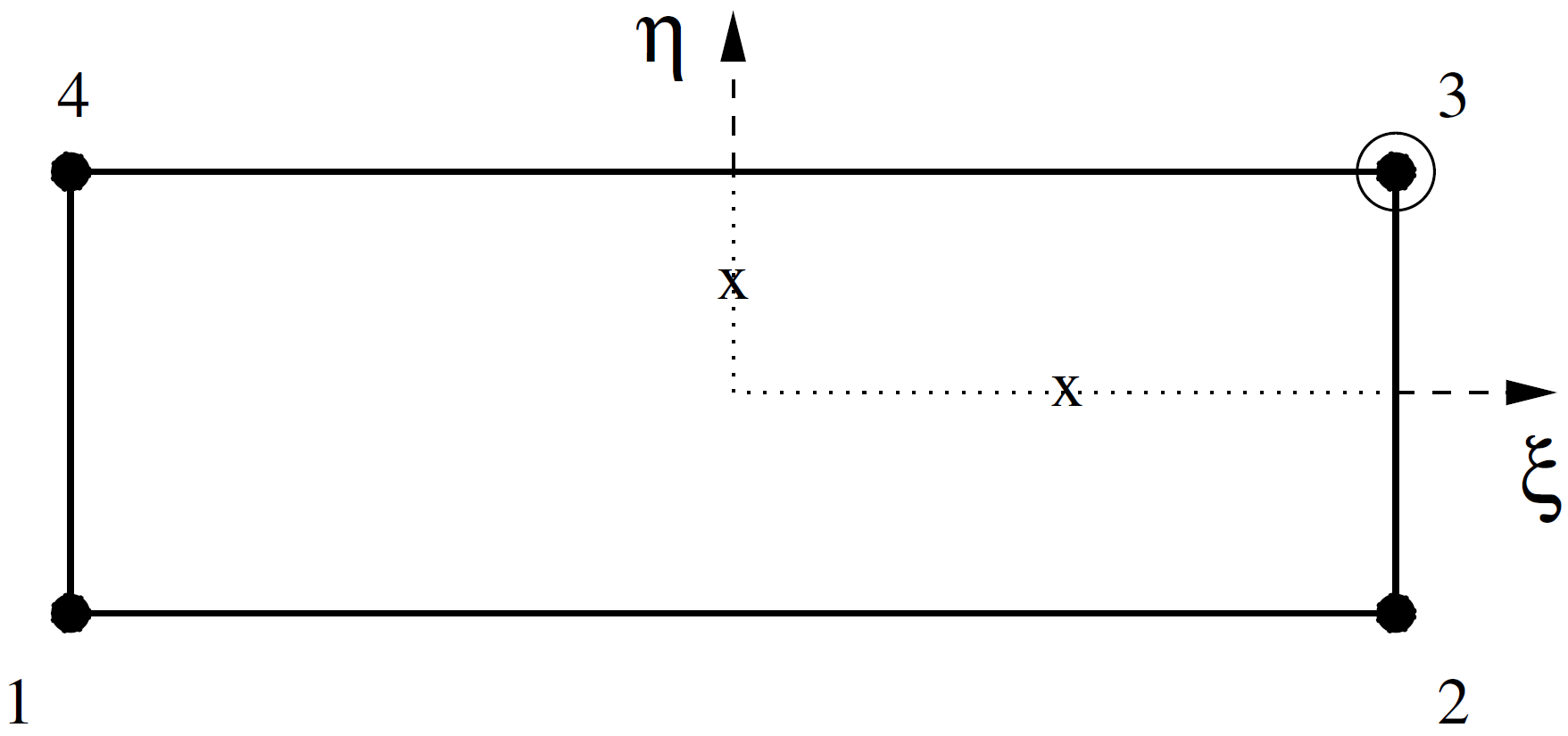
Fig. 3.42 Control volume faces in a single element. Contributions to the the control volume centered about node 3.
Integration point shift functions and the critical aspect ratio are derived for isoparametric quadrilateral elements with bilinear shape functions, and hexahedral elements with trilinear shape functions. Only the orthogonal form is considered. Linear triangles are discussed since they can also produce negative coefficients. For linear elements, only the element geometry (mesh quality) can be modified to control negative coefficients. With isoparametric bilinear and trilinear elements, both the geometry and the location of the integration point control negativity. In addition, integration point shifting is compared to finite-element hour-glass control. Positive coefficients are achieved by either shifting the element integration points or applying the hour-glass stabilization matrix, and in some cases the two are identical.
3.4.10.1.1. Aspect Ratio Definition
In this section, the isoparametric coordinates for an element are oriented such that the aspect ratio is greater than or equal to one. In two dimensions, the aspect ratio for an orthogonal element is the ratio between edge lengths. In three dimensions, each element has two aspect ratios since there are potentially three different edge lengths. The aspect ratios are taken relative to the shortest of the edge lengths which has a reference length of one.
3.4.10.1.2. Quadrilateral Elements
The coefficients for the diffusion operator result from the combination of two basic second-order accurate diffusion operators: the edge operator and the centroid operator, shown in Figure 3.43. The two operators represent the extremes in evaluating derivatives using the bilinear shape function within the element. The edge scheme always gives positive coefficients while the centroid scheme gives rise to negative coefficients above a certain aspect ratio. The centroid scheme results from evaluating all the derivatives for the four control volume sub-faces at the element centroid, equivalent to reduced integration [237] in GFEM. The edge scheme results from evaluating the derivatives out at the ends of the sub-faces in CVFEM or out at the nodes in GFEM. The edge scheme returns the standard five-point finite-difference operator. The traditional CVFEM [159] uses an equal weighting of the edge and the centroid scheme. The GFEM uses one part edge to two parts centroid.
The GFEM is more prone to oscillations with high aspect ratio elements than the CVFEM because it contains a larger weighting of the centroid scheme. The single-point-integrated GFEM element will be the most unstable since it is a pure centroid scheme.
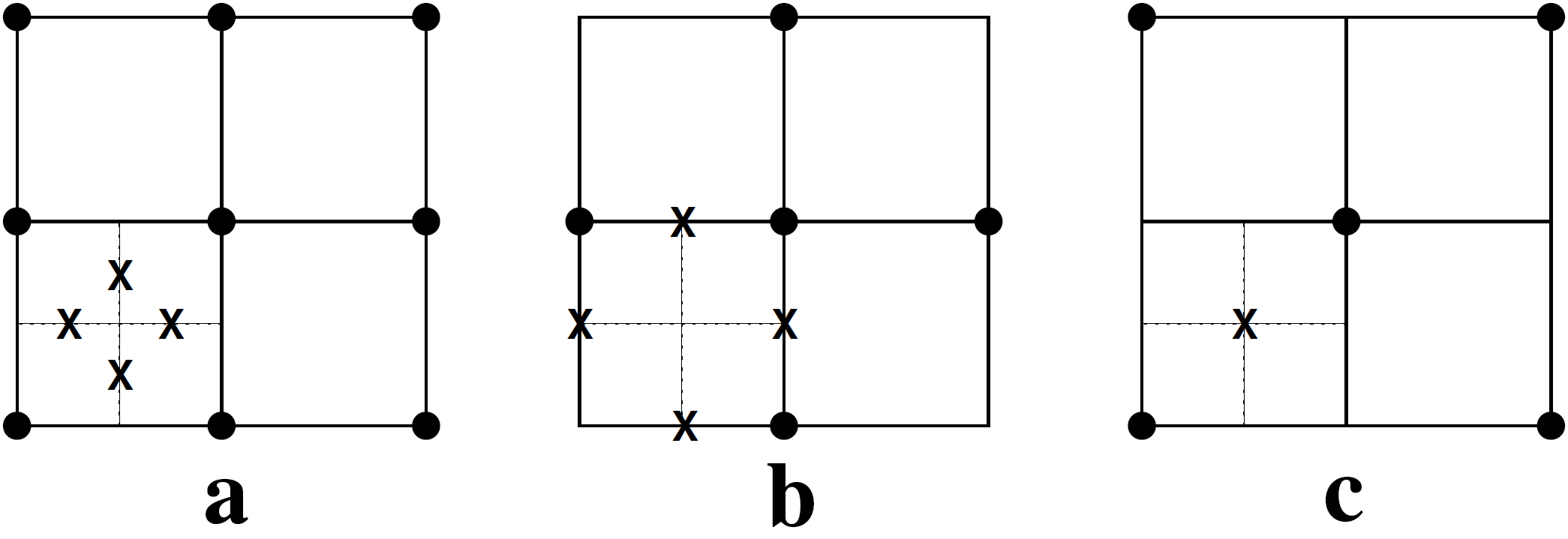
Fig. 3.43 Flux integration points (X) determine nodal ( ) contributions to the coefficient
stencil: a) mid-face rule of CVFEM, b) edge–operator, c) centroid–operator (one-point integration).
) contributions to the coefficient
stencil: a) mid-face rule of CVFEM, b) edge–operator, c) centroid–operator (one-point integration).
The coefficient signs for a rectangular element are controlled by
moving the integration points away from the centroid of the element.
The smallest value of the integration point shift
that satisfies coefficient positivity is found by symbolically
integrating the diffusion flux over a control volume.
Consider the diffusion operator evaluated over a
collection of equal-size rectangular elements.
Each element is longer by a factor of  in the
x-direction than the y-direction, where is the aspect
ratio of the elements.
The integration points can be shifted in
the
in the
x-direction than the y-direction, where is the aspect
ratio of the elements.
The integration points can be shifted in
the  -direction by
  and in the
  -direction by
  .
The element coefficients that contribute to the
equation centered at Node 3 in Fig. Control volume faces in a single element. Contributions to the the control volume centered about node 3. are:
.
The element coefficients that contribute to the
equation centered at Node 3 in Fig. Control volume faces in a single element. Contributions to the the control volume centered about node 3. are:
(3.1146)
(3.1147)
(3.1148)
(3.1149)
The positivity constraint for Node 3 comes from coefficient 4
in the element matrix, where the
coefficient becomes negative for large values of aspect
ratio. The -shift removes the effect of aspect ratio,
while the -shift has no effect on negativity.
For CVFEM, the integration points on vertical
faces, in the longer x-direction, should be shifted from the mid-faces
out towards the element edges by .
The y-direction flux is the only flux effected by the shift
so the y-direction flux is the flux associated with negative
coefficients. The minimal amount of -shift required to
maintain positivity depends upon the aspect ratio,
(3.1150)
The maximum aspect ratio for which the unshifted CVFEM remains
monotone is .
A similar formula exists for GFEM, where and are
shifted from the Gauss points at  .
The element coefficients that contribute to the
equation centered at Node 3 in Fig. Control volume faces in a single element. Contributions to the the control volume centered about node 3. are:
.
The element coefficients that contribute to the
equation centered at Node 3 in Fig. Control volume faces in a single element. Contributions to the the control volume centered about node 3. are:
(3.1151)
(3.1152)
(3.1153)
(3.1154)
Similar to the CVFEM, the -shift is the only shift that
affects the aspect ratio term.
The positivity constraint for Node 3 comes from coefficient 4 in
the element matrix,
(3.1155)
The maximum aspect ratio for which the unshifted GFEM remains
monotone is .
The shift values are very sensitive to the aspect ratio, out to an aspect ratio of about four. The values of the integration point shift function are plotted as a function of the aspect ratio in Figure 3.44. At that aspect ratio, the shifted integration points are near the edge of the element. Since the requisite integration point shift rapidly reaches the element edge for increasing aspect ratio, it can be argued that the maximum shift should always be taken. It will be shown in the section on accuracy that integration point shifting leads to a general loss in accuracy on non-orthogonal meshes. Therefore, it may be desirable to use (3.1150) to compute the minimal shift for each element. The accuracy consideration must be traded against the algorithmic complexity of computing geometry-dependent shape functions for each element.
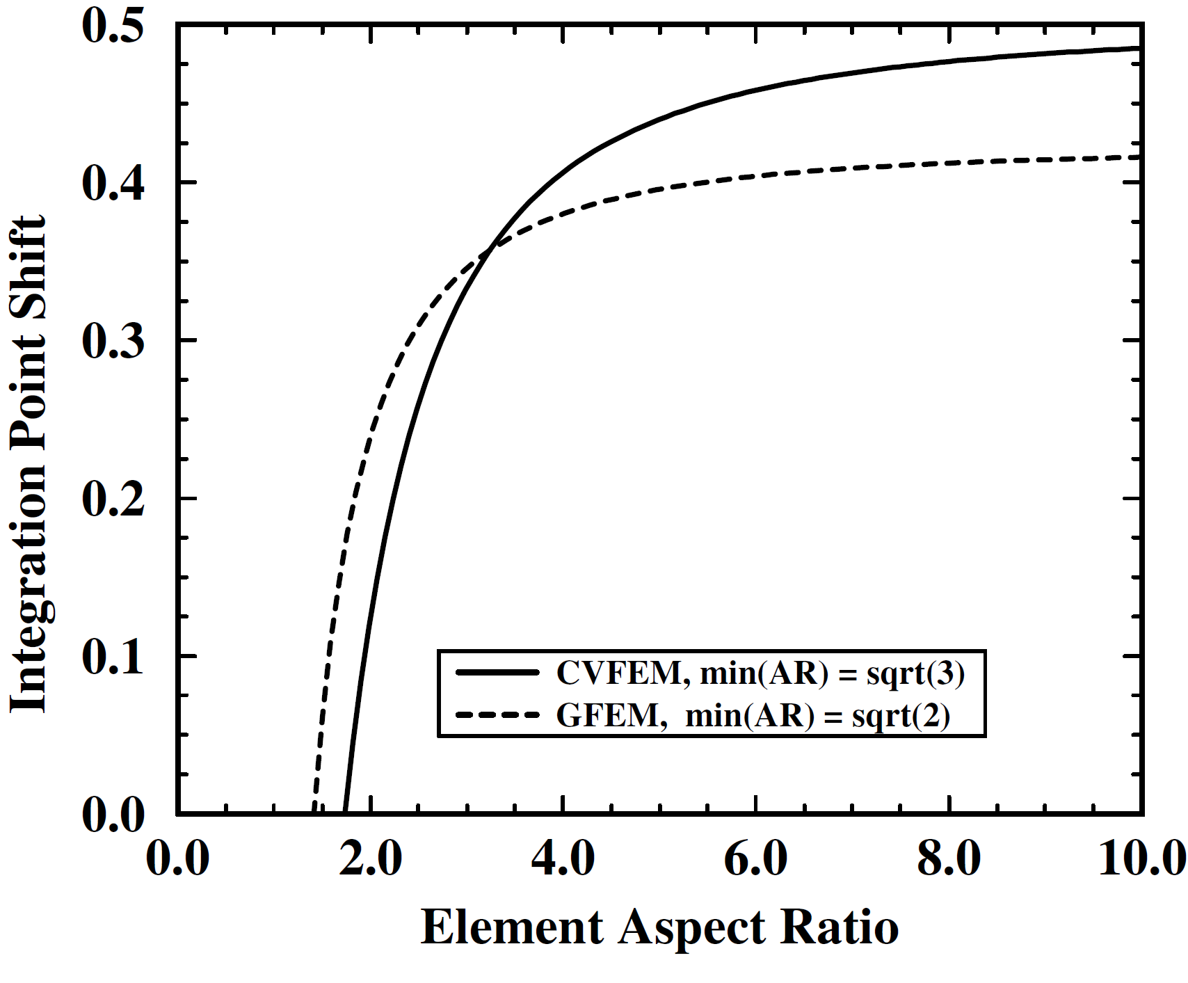
Fig. 3.44 Integration point locations must be shifted out towards the element-edge with increasing element aspect ratio.
3.4.10.1.3. Reduced Integration
One-point integration methods for quadrilateral and hexahedral elements are popular because they are computationally efficient. Sometimes, oscillations occur and are called hour-glass modes after the displaced element shapes. Hour-glass stabilization methods prevent the hour-glass oscillations from occurring. The hour-glass terms are derived by examining the eigenmodes of the finite-elements and noting that there are missing mode shapes when the elements are integrated at the center [237]. The stabilization term adds the effects of the missing mode shapes back into the element formulation.
It is shown here that the hour-glass stabilization terms have the same effect on the element coefficients as shifting the integration points in two-dimensional elements. Both the hour-glass stabilization and the integration-point shifting modify the discretization to look more like a five-point scheme; or, more like the edge scheme of the previous section. The H-stabilization method is commonly used [130] in the GFEM with reduced integration. For quadrilateral elements, the element matrix for the hour-glass stabilization term is
(3.1156)![C_{\rm hg} \left[
\begin{array}{rrrr}
-1 1 -1 1 \\
1 -1 1 -1 \\
-1 1 -1 1 \\
1 -1 1 -1
\end{array}
\right],](data:image/svg+xml;base64,PD94bWwgdmVyc2lvbj0nMS4wJyBlbmNvZGluZz0nVVRGLTgnPz4KPCEtLSBUaGlzIGZpbGUgd2FzIGdlbmVyYXRlZCBieSBkdmlzdmdtIDMuMC4zIC0tPgo8c3ZnIHZlcnNpb249JzEuMScgeG1sbnM9J2h0dHA6Ly93d3cudzMub3JnLzIwMDAvc3ZnJyB4bWxuczp4bGluaz0naHR0cDovL3d3dy53My5vcmcvMTk5OS94bGluaycgd2lkdGg9JzExOS4xMjEwNjJwdCcgaGVpZ2h0PSc2Ni45NDk2MDdwdCcgdmlld0JveD0nMTM0LjcxMDk0NCAtNjcuMzQ3Nzc2IDExOS4xMjEwNjIgNjYuOTQ5NjA3Jz4KPGRlZnM+CjxwYXRoIGlkPSdnMS0wJyBkPSdNOS4xOTE1MzItMy4yMDc5N0M5LjQyODY0My0zLjIwNzk3IDkuNjc5NzAxLTMuMjA3OTcgOS42Nzk3MDEtMy40ODY5MjRTOS40Mjg2NDMtMy43NjU4NzggOS4xOTE1MzItMy43NjU4NzhIMS42NDU4MjhDMS40MDg3MTctMy43NjU4NzggMS4xNTc2NTktMy43NjU4NzggMS4xNTc2NTktMy40ODY5MjRTMS40MDg3MTctMy4yMDc5NyAxLjY0NTgyOC0zLjIwNzk3SDkuMTkxNTMyWicvPgo8cGF0aCBpZD0nZzQtNDknIGQ9J000LjAxNjkzNi04Ljk0MDQ3M0M0LjAxNjkzNi05LjI2MTI3IDQuMDE2OTM2LTkuMjc1MjE4IDMuNzM3OTgzLTkuMjc1MjE4QzMuNDAzMjM4LTguODk4NjMgMi43MDU4NTMtOC4zODI1NjUgMS4yNjkyNC04LjM4MjU2NVYtNy45NzgwODJDMS41OTAwMzctNy45NzgwODIgMi4yODc0MjItNy45NzgwODIgMy4wNTQ1NDUtOC4zNDA3MjJWLTEuMDczOTczQzMuMDU0NTQ1LS41NzE4NTYgMy4wMTI3MDItLjQwNDQ4MyAxLjc4NTMwNS0uNDA0NDgzSDEuMzUyOTI3VjBDMS43Mjk1MTQtLjAyNzg5NSAzLjA4MjQ0MS0uMDI3ODk1IDMuNTQyNzE1LS4wMjc4OTVTNS4zNDE5NjgtLjAyNzg5NSA1LjcxODU1NSAwVi0uNDA0NDgzSDUuMjg2MTc3QzQuMDU4NzgtLjQwNDQ4MyA0LjAxNjkzNi0uNTcxODU2IDQuMDE2OTM2LTEuMDczOTczVi04Ljk0MDQ3M1onLz4KPHBhdGggaWQ9J2cwLTUwJyBkPSdNNC41NDY5NDkgMjQuNTQ3OTQ1SDUuNTA5MzRWLjQxODQzMUg5LjE5MTUzMlYtLjU0Mzk2SDQuNTQ2OTQ5VjI0LjU0Nzk0NVonLz4KPHBhdGggaWQ9J2cwLTUxJyBkPSdNMy43Nzk4MjYgMjQuNTQ3OTQ1SDQuNzQyMjE3Vi0uNTQzOTZILjA5NzYzNFYuNDE4NDMxSDMuNzc5ODI2VjI0LjU0Nzk0NVonLz4KPHBhdGggaWQ9J2cwLTUyJyBkPSdNNC41NDY5NDkgMjQuNTMzOTk4SDkuMTkxNTMyVjIzLjU3MTYwNkg1LjUwOTM0Vi0uNTU3OTA4SDQuNTQ2OTQ5VjI0LjUzMzk5OFonLz4KPHBhdGggaWQ9J2cwLTUzJyBkPSdNMy43Nzk4MjYgMjMuNTcxNjA2SC4wOTc2MzRWMjQuNTMzOTk4SDQuNzQyMjE3Vi0uNTU3OTA4SDMuNzc5ODI2VjIzLjU3MTYwNlonLz4KPHBhdGggaWQ9J2cwLTU0JyBkPSdNNC41NDY5NDkgOC4zODI1NjVINS41MDkzNFYtLjAxMzk0OEg0LjU0Njk0OVY4LjM4MjU2NVonLz4KPHBhdGggaWQ9J2cwLTU1JyBkPSdNMy43Nzk4MjYgOC4zODI1NjVINC43NDIyMTdWLS4wMTM5NDhIMy43Nzk4MjZWOC4zODI1NjVaJy8+CjxwYXRoIGlkPSdnMi01OScgZD0nTTIuNzE5ODAxIC4wNTU3OTFDMi43MTk4MDEtLjc1MzE3NiAyLjQ1NDc5NS0xLjM1MjkyNyAxLjg4MjkzOS0xLjM1MjkyN0MxLjQzNjYxMy0xLjM1MjkyNyAxLjIxMzQ1LS45OTAyODYgMS4yMTM0NS0uNjgzNDM3UzEuNDIyNjY1IDAgMS44OTY4ODcgMEMyLjA3ODIwNyAwIDIuMjMxNjMxLS4wNTU3OTEgMi4zNTcxNjEtLjE4MTMyQzIuMzg1MDU2LS4yMDkyMTUgMi4zOTkwMDQtLjIwOTIxNSAyLjQxMjk1MS0uMjA5MjE1QzIuNDQwODQ3LS4yMDkyMTUgMi40NDA4NDctLjAxMzk0OCAyLjQ0MDg0NyAuMDU1NzkxQzIuNDQwODQ3IC41MTYwNjUgMi4zNTcxNjEgMS40MjI2NjUgMS41NDgxOTQgMi4zMjkyNjVDMS4zOTQ3NyAyLjQ5NjYzOCAxLjM5NDc3IDIuNTI0NTMzIDEuMzk0NzcgMi41NTI0MjhDMS4zOTQ3NyAyLjYyMjE2NyAxLjQ2NDUwOCAyLjY5MTkwNSAxLjUzNDI0NyAyLjY5MTkwNUMxLjY0NTgyOCAyLjY5MTkwNSAyLjcxOTgwMSAxLjY1OTc3NiAyLjcxOTgwMSAuMDU1NzkxWicvPgo8cGF0aCBpZD0nZzItNjcnIGQ9J00xMC40MTg5MjktOS42OTM2NDlDMTAuNDE4OTI5LTkuODE5MTc4IDEwLjMyMTI5NS05LjgxOTE3OCAxMC4yOTM0LTkuODE5MTc4UzEwLjIwOTcxNC05LjgxOTE3OCAxMC4wOTgxMzItOS42Nzk3MDFMOS4xMzU3NDEtOC41MDgwOTVDOC42NDc1NzItOS4zNDQ5NTYgNy44ODA0NDgtOS44MTkxNzggNi44MzQzNzEtOS44MTkxNzhDMy44MjE2NjktOS44MTkxNzggLjY5NzM4NS02Ljc2NDYzMyAuNjk3Mzg1LTMuNDg2OTI0Qy42OTczODUtMS4xNTc2NTkgMi4zMjkyNjUgLjI5MjkwMiA0LjM2NTYyOSAuMjkyOTAyQzUuNDgxNDQ1IC4yOTI5MDIgNi40NTc3ODMtLjE4MTMyIDcuMjY2NzUtLjg2NDc1N0M4LjQ4MDE5OS0xLjg4MjkzOSA4Ljg0MjgzOS0zLjIzNTg2NiA4Ljg0MjgzOS0zLjM0NzQ0N0M4Ljg0MjgzOS0zLjQ3Mjk3NiA4LjczMTI1OC0zLjQ3Mjk3NiA4LjY4OTQxNS0zLjQ3Mjk3NkM4LjU2Mzg4NS0zLjQ3Mjk3NiA4LjU0OTkzOC0zLjM4OTI5IDguNTIyMDQyLTMuMzMzNDk5QzcuODgwNDQ4LTEuMTU3NjU5IDUuOTk3NTA5LS4xMTE1ODIgNC42MDI3NC0uMTExNTgyQzMuMTI0Mjg0LS4xMTE1ODIgMS44NDEwOTYtMS4wNjAwMjUgMS44NDEwOTYtMy4wNDA1OThDMS44NDEwOTYtMy40ODY5MjQgMS45ODA1NzMtNS45MTM4MjMgMy41NTY2NjMtNy43NDA5NzFDNC4zMjM3ODYtOC42MzM2MjQgNS42MzQ4NjktOS40MTQ2OTUgNi45NTk5LTkuNDE0Njk1QzguNDk0MTQ3LTkuNDE0Njk1IDkuMTc3NTg0LTguMTQ1NDU1IDkuMTc3NTg0LTYuNzIyNzlDOS4xNzc1ODQtNi4zNjAxNDkgOS4xMzU3NDEtNi4wNTMzIDkuMTM1NzQxLTUuOTk3NTA5QzkuMTM1NzQxLTUuODcxOTggOS4yNzUyMTgtNS44NzE5OCA5LjMxNzA2MS01Ljg3MTk4QzkuNDcwNDg2LTUuODcxOTggOS40ODQ0MzMtNS44ODU5MjggOS41NDAyMjQtNi4xMzY5ODZMMTAuNDE4OTI5LTkuNjkzNjQ5WicvPgo8cGF0aCBpZD0nZzMtMTAzJyBkPSdNMi4xNjc0NjMtMS42NzkyOTVDMS4zMTgwNTItMS42NzkyOTUgMS4zMTgwNTItMi42NTU2MyAxLjMxODA1Mi0yLjg4MDE4N0MxLjMxODA1Mi0zLjE0Mzc5NyAxLjMyNzgxNS0zLjQ1NjIyNCAxLjQ3NDI2NS0zLjcwMDMwOEMxLjU1MjM3Mi0zLjgxNzQ2OCAxLjc3NjkyOS00LjA5MDg0MSAyLjE2NzQ2My00LjA5MDg0MUMzLjAxNjg3NC00LjA5MDg0MSAzLjAxNjg3NC0zLjExNDUwNyAzLjAxNjg3NC0yLjg4OTk1QzMuMDE2ODc0LTIuNjI2MzQgMy4wMDcxMS0yLjMxMzkxMyAyLjg2MDY2LTIuMDY5ODI5QzIuNzgyNTUzLTEuOTUyNjY5IDIuNTU3OTk2LTEuNjc5Mjk1IDIuMTY3NDYzLTEuNjc5Mjk1Wk0xLjAzNDkxNS0xLjI5ODUyNUMxLjAzNDkxNS0xLjMzNzU3OCAxLjAzNDkxNS0xLjU2MjEzNSAxLjIwMDg5MS0xLjc1NzQwMkMxLjU4MTY2Mi0xLjQ4NDAyOCAxLjk4MTk1OS0xLjQ1NDczOCAyLjE2NzQ2My0xLjQ1NDczOEMzLjA3NTQ1NC0xLjQ1NDczOCAzLjc0OTEyNC0yLjEyODQwOSAzLjc0OTEyNC0yLjg4MDE4N0MzLjc0OTEyNC0zLjI0MTQzIDMuNTkyOTExLTMuNjAyNjc0IDMuMzQ4ODI3LTMuODI3MjMxQzMuNzAwMzA4LTQuMTU5MTg1IDQuMDUxNzg4LTQuMjA4MDAyIDQuMjI3NTI4LTQuMjA4MDAyQzQuMjQ3MDU1LTQuMjA4MDAyIDQuMjk1ODcyLTQuMjA4MDAyIDQuMzI1MTYyLTQuMTk4MjM4QzQuMjE3NzY1LTQuMTU5MTg1IDQuMTY4OTQ4LTQuMDUxNzg4IDQuMTY4OTQ4LTMuOTM0NjI4QzQuMTY4OTQ4LTMuNzY4NjUxIDQuMjk1ODcyLTMuNjUxNDkxIDQuNDUyMDg1LTMuNjUxNDkxQzQuNTQ5NzE5LTMuNjUxNDkxIDQuNzM1MjIyLTMuNzE5ODM0IDQuNzM1MjIyLTMuOTQ0MzkxQzQuNzM1MjIyLTQuMTEwMzY4IDQuNjE4MDYyLTQuNDIyNzk1IDQuMjM3MjkyLTQuNDIyNzk1QzQuMDQyMDI1LTQuNDIyNzk1IDMuNjEyNDM4LTQuMzY0MjE1IDMuMjAyMzc3LTMuOTYzOTE4QzIuNzkyMzE3LTQuMjg2MTA4IDIuMzgyMjU2LTQuMzE1Mzk4IDIuMTY3NDYzLTQuMzE1Mzk4QzEuMjU5NDcxLTQuMzE1Mzk4IC41ODU4MDEtMy42NDE3MjggLjU4NTgwMS0yLjg4OTk1Qy41ODU4MDEtMi40NjAzNjMgLjgwMDU5NC0yLjA4OTM1NiAxLjA0NDY3OC0xLjg4NDMyNkMuOTE3NzU0LTEuNzM3ODc1IC43NDIwMTQtMS40MTU2ODUgLjc0MjAxNC0xLjA3Mzk2OEMuNzQyMDE0LS43NzEzMDQgLjg2ODkzOC0uNDAwMjk3IDEuMTcxNjAxLS4yMDUwM0MuNTg1ODAxLS4wMzkwNTMgLjI3MzM3NCAuMzgwNzcgLjI3MzM3NCAuNzcxMzA0Qy4yNzMzNzQgMS40NzQyNjUgMS4yMzk5NDUgMi4wMTEyNDkgMi40MzEwNzMgMi4wMTEyNDlDMy41ODMxNDggMi4wMTEyNDkgNC41OTg1MzUgMS41MTMzMTggNC41OTg1MzUgLjc1MTc3OEM0LjU5ODUzNSAuNDEwMDYgNC40NjE4NDktLjA4Nzg3IDMuOTYzOTE4LS4zNjEyNDRDMy40NDY0NjEtLjYzNDYxNyAyLjg4MDE4Ny0uNjM0NjE3IDIuMjg0NjIzLS42MzQ2MTdDMi4wNDA1MzktLjYzNDYxNyAxLjYyMDcxNS0uNjM0NjE3IDEuNTUyMzcyLS42NDQzODFDMS4yMzk5NDUtLjY4MzQzNCAxLjAzNDkxNS0uOTg2MDk4IDEuMDM0OTE1LTEuMjk4NTI1Wk0yLjQ0MDgzNiAxLjc4NjY5MkMxLjQ1NDczOCAxLjc4NjY5MiAuNzgxMDY4IDEuMjg4NzYyIC43ODEwNjggLjc3MTMwNEMuNzgxMDY4IC4zMjIxOSAxLjE1MjA3NS0uMDM5MDUzIDEuNTgxNjYyLS4wNjgzNDNIMi4xNTc2OTlDMi45OTczNDctLjA2ODM0MyA0LjA5MDg0MS0uMDY4MzQzIDQuMDkwODQxIC43NzEzMDRDNC4wOTA4NDEgMS4yOTg1MjUgMy4zOTc2NDQgMS43ODY2OTIgMi40NDA4MzYgMS43ODY2OTJaJy8+CjxwYXRoIGlkPSdnMy0xMDQnIGQ9J00xLjA3Mzk2OC0uNzQyMDE0QzEuMDczOTY4LS4zMDI2NjQgLjk2NjU3MS0uMzAyNjY0IC4zMTI0MjctLjMwMjY2NFYwQy42NTQxNDQtLjAwOTc2MyAxLjE1MjA3NS0uMDI5MjkgMS40MTU2ODUtLjAyOTI5QzEuNjY5NTMyLS4wMjkyOSAyLjE3NzIyNi0uMDA5NzYzIDIuNTA5MTggMFYtLjMwMjY2NEMxLjg1NTAzNS0uMzAyNjY0IDEuNzQ3NjM5LS4zMDI2NjQgMS43NDc2MzktLjc0MjAxNFYtMi41Mzg0N0MxLjc0NzYzOS0zLjU1Mzg1NyAyLjQ0MDgzNi00LjEwMDYwNSAzLjA2NTY5LTQuMTAwNjA1QzMuNjgwNzgxLTQuMTAwNjA1IDMuNzg4MTc4LTMuNTczMzg0IDMuNzg4MTc4LTMuMDE2ODc0Vi0uNzQyMDE0QzMuNzg4MTc4LS4zMDI2NjQgMy42ODA3ODEtLjMwMjY2NCAzLjAyNjYzNy0uMzAyNjY0VjBDMy4zNjgzNTQtLjAwOTc2MyAzLjg2NjI4NS0uMDI5MjkgNC4xMjk4OTUtLjAyOTI5QzQuMzgzNzQyLS4wMjkyOSA0Ljg5MTQzNi0uMDA5NzYzIDUuMjIzMzg5IDBWLS4zMDI2NjRDNC43MTU2OTYtLjMwMjY2NCA0LjQ3MTYxMi0uMzAyNjY0IDQuNDYxODQ5LS41OTU1NjRWLTIuNDYwMzYzQzQuNDYxODQ5LTMuMzAwMDExIDQuNDYxODQ5LTMuNjAyNjc0IDQuMTU5MTg1LTMuOTU0MTU1QzQuMDIyNDk4LTQuMTIwMTMxIDMuNzAwMzA4LTQuMzE1Mzk4IDMuMTM0MDM0LTQuMzE1Mzk4QzIuMzEzOTEzLTQuMzE1Mzk4IDEuODg0MzI2LTMuNzI5NTk4IDEuNzE4MzQ5LTMuMzU4NTkxVi02Ljc3NTc2MUwuMzEyNDI3LTYuNjY4MzY0Vi02LjM2NTcwMUMuOTk1ODYxLTYuMzY1NzAxIDEuMDczOTY4LTYuMjk3MzU3IDEuMDczOTY4LTUuODE4OTUzVi0uNzQyMDE0WicvPgo8L2RlZnM+CjxnIGlkPSdwYWdlMSc+Cjx1c2UgeD0nMTM0LjcxMDk0NCcgeT0nLTMwLjM4NjA1MicgeGxpbms6aHJlZj0nI2cyLTY3Jy8+Cjx1c2UgeD0nMTQ0LjQ4MTgzMScgeT0nLTI4LjI5MzkwNycgeGxpbms6aHJlZj0nI2czLTEwNCcvPgo8dXNlIHg9JzE0OS45MDU5MjgnIHk9Jy0yOC4yOTM5MDcnIHhsaW5rOmhyZWY9JyNnMy0xMDMnLz4KPHVzZSB4PScxNTcuNzQ1OTE4JyB5PSctNjYuNzg5ODgyJyB4bGluazpocmVmPScjZzAtNTAnLz4KPHVzZSB4PScxNTcuNzQ1OTE4JyB5PSctNDIuMjQxNjc5JyB4bGluazpocmVmPScjZzAtNTQnLz4KPHVzZSB4PScxNTcuNzQ1OTE4JyB5PSctMzMuODcyOTc2JyB4bGluazpocmVmPScjZzAtNTQnLz4KPHVzZSB4PScxNTcuNzQ1OTE4JyB5PSctMjQuOTQ2MzgzJyB4bGluazpocmVmPScjZzAtNTInLz4KPHVzZSB4PScxNzguMjI0NjUnIHk9Jy01NS44OTA0NjMnIHhsaW5rOmhyZWY9JyNnMS0wJy8+Cjx1c2UgeD0nMTg5LjA3Mjg5NicgeT0nLTU1Ljg5MDQ2MycgeGxpbms6aHJlZj0nI2c0LTQ5Jy8+Cjx1c2UgeD0nMTk1LjkwMTM4NScgeT0nLTU1Ljg5MDQ2MycgeGxpbms6aHJlZj0nI2c0LTQ5Jy8+Cjx1c2UgeD0nMjA1LjgyOTMzNCcgeT0nLTU1Ljg5MDQ2MycgeGxpbms6aHJlZj0nI2cxLTAnLz4KPHVzZSB4PScyMTkuNzc3MDQyJyB5PSctNTUuODkwNDYzJyB4bGluazpocmVmPScjZzQtNDknLz4KPHVzZSB4PScyMjYuNjA1NTMxJyB5PSctNTUuODkwNDYzJyB4bGluazpocmVmPScjZzQtNDknLz4KPHVzZSB4PScxNzIuMDI1NzI4JyB5PSctMzguOTUzOTc0JyB4bGluazpocmVmPScjZzQtNDknLz4KPHVzZSB4PScxODEuOTUzNjc3JyB5PSctMzguOTUzOTc0JyB4bGluazpocmVmPScjZzEtMCcvPgo8dXNlIHg9JzE5NS45MDEzODUnIHk9Jy0zOC45NTM5NzQnIHhsaW5rOmhyZWY9JyNnNC00OScvPgo8dXNlIHg9JzIwMi43Mjk4NzMnIHk9Jy0zOC45NTM5NzQnIHhsaW5rOmhyZWY9JyNnNC00OScvPgo8dXNlIHg9JzIxMi42NTc4MjMnIHk9Jy0zOC45NTM5NzQnIHhsaW5rOmhyZWY9JyNnMS0wJy8+Cjx1c2UgeD0nMjI2LjYwNTUzMScgeT0nLTM4Ljk1Mzk3NCcgeGxpbms6aHJlZj0nI2c0LTQ5Jy8+Cjx1c2UgeD0nMTc4LjIyNDY1JyB5PSctMjIuMDE3NDg2JyB4bGluazpocmVmPScjZzEtMCcvPgo8dXNlIHg9JzE4OS4wNzI4OTYnIHk9Jy0yMi4wMTc0ODYnIHhsaW5rOmhyZWY9JyNnNC00OScvPgo8dXNlIHg9JzE5NS45MDEzODUnIHk9Jy0yMi4wMTc0ODYnIHhsaW5rOmhyZWY9JyNnNC00OScvPgo8dXNlIHg9JzIwNS44MjkzMzQnIHk9Jy0yMi4wMTc0ODYnIHhsaW5rOmhyZWY9JyNnMS0wJy8+Cjx1c2UgeD0nMjE5Ljc3NzA0MicgeT0nLTIyLjAxNzQ4NicgeGxpbms6aHJlZj0nI2c0LTQ5Jy8+Cjx1c2UgeD0nMjI2LjYwNTUzMScgeT0nLTIyLjAxNzQ4NicgeGxpbms6aHJlZj0nI2c0LTQ5Jy8+Cjx1c2UgeD0nMTcyLjAyNTcyOCcgeT0nLTUuMDgwOTk4JyB4bGluazpocmVmPScjZzQtNDknLz4KPHVzZSB4PScxODEuOTUzNjc3JyB5PSctNS4wODA5OTgnIHhsaW5rOmhyZWY9JyNnMS0wJy8+Cjx1c2UgeD0nMTk1LjkwMTM4NScgeT0nLTUuMDgwOTk4JyB4bGluazpocmVmPScjZzQtNDknLz4KPHVzZSB4PScyMDIuNzI5ODczJyB5PSctNS4wODA5OTgnIHhsaW5rOmhyZWY9JyNnNC00OScvPgo8dXNlIHg9JzIxMi42NTc4MjMnIHk9Jy01LjA4MDk5OCcgeGxpbms6aHJlZj0nI2cxLTAnLz4KPHVzZSB4PScyMjYuNjA1NTMxJyB5PSctNS4wODA5OTgnIHhsaW5rOmhyZWY9JyNnNC00OScvPgo8dXNlIHg9JzIzOC40MTUzMTYnIHk9Jy02Ni43ODk4ODInIHhsaW5rOmhyZWY9JyNnMC01MScvPgo8dXNlIHg9JzIzOC40MTUzMTYnIHk9Jy00Mi4yNDE2NzknIHhsaW5rOmhyZWY9JyNnMC01NScvPgo8dXNlIHg9JzIzOC40MTUzMTYnIHk9Jy0zMy44NzI5NzYnIHhsaW5rOmhyZWY9JyNnMC01NScvPgo8dXNlIHg9JzIzOC40MTUzMTYnIHk9Jy0yNC45NDYzODMnIHhsaW5rOmhyZWY9JyNnMC01MycvPgo8dXNlIHg9JzI1MC4wMzg0MDInIHk9Jy0zMC4zODYwNTInIHhsaW5rOmhyZWY9JyNnMi01OScvPgo8L2c+Cjwvc3ZnPgo8IS0tIERFUFRIPTAgLS0+)
where the constant  contains scaling information.
The first row of the hour-glass stabilization matrix,
(3.1156), can also be derived by subtracting the
matrix coefficients for the one-point integrated GFEM,
(3.1157),
contains scaling information.
The first row of the hour-glass stabilization matrix,
(3.1156), can also be derived by subtracting the
matrix coefficients for the one-point integrated GFEM,
(3.1157),
(3.1157)
from the coefficients for the five-point difference scheme, (3.1158),
(3.1158)
The resulting coefficient set is identical to the
hour-glass stabilization matrix,
(3.1156), if the multiplier
 . The hour-glass
stabilization matrix is added to a diffusion operator to
make it look more like a five-point finite difference scheme.
Note that the multiplier used by GFEM practitioners [130]
is
. The hour-glass
stabilization matrix is added to a diffusion operator to
make it look more like a five-point finite difference scheme.
Note that the multiplier used by GFEM practitioners [130]
is  .
The hour-glass
stabilization matrix can also be used with other schemes.
The multiplier for standard GFEM is
.
The hour-glass
stabilization matrix can also be used with other schemes.
The multiplier for standard GFEM is
 .
The multiplier for standard CVFEM is
.
The multiplier for standard CVFEM is
 ,
though conservation is only guaranteed on rectangular meshes.
,
though conservation is only guaranteed on rectangular meshes.
3.4.10.1.4. Triangular Elements
Linear triangular elements can also produce negative off-diagonal coefficients.
There are no shift-functions for triangles since the gradients are constant over the element. Negative coefficients result from the geometry of the element.
Nodal coefficients for a triangular element are computed for the diffusion flux contributions, shown in Figure 3.45. The nodal coefficients for the diffusion flux contribution to the control volume centered about Node 1 are
(3.1159)
(3.1160)
(3.1161)
where the base edge length is  and the two adjacent vertex
angles are
and the two adjacent vertex
angles are  and
and  .
The conditions required to ensure that all the off-diagonal terms remain
positive are combined from constraints on all three control volume
contributions,
.
The conditions required to ensure that all the off-diagonal terms remain
positive are combined from constraints on all three control volume
contributions,
(3.1162)
(3.1163)
(3.1164)
The triangular element yields positive off-diagonal coefficients
if  ,
,  , and
, and
 . The triangle must be acute.
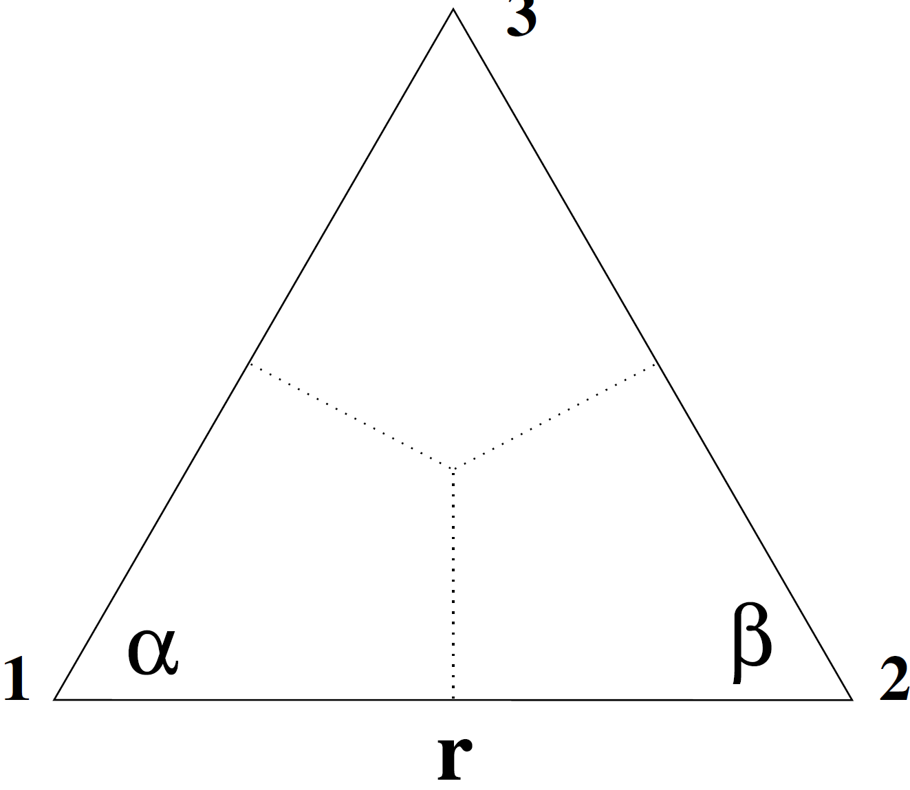
Fig. 3.45 Triangular element geometry in defined by edge length and two vertex angles.
In a previous work [204], quadrilateral elements were subdivided into triangular elements using edge-swapping, along with a Delaunay algorithm, to minimize the effect of negative coefficients. Given a collection of nodes, a Delaunay triangulation of the nodes will generate triangles where the minimum angle between vertices is maximized, leading to near-equilateral triangles that satisfy (3.1162).
3.4.10.1.5. Hex Elements
The aspect ratio limit for the CVFEM diffusion
operator with orthogonal, hexahedral elements can be as large as
if the base is square. The three-dimensional
element is more difficult to control because there are two aspect ratios.
The local element node numbering for a hexahedron is defined
in Fig. Hexahedral element topology and numbering. Let the edge length between Nodes 1 and 2 be
of value  , the edge length between Nodes 1 and 4 be of value
  ,
and the edge length between Nodes 1 and 5 be of value
,
and the edge length between Nodes 1 and 5 be of value  .
These are the , , and
.
These are the , , and  directions.
The parametric representation of the nodal coefficients for
the element contribution to the control volume centered about
Node 1 is
directions.
The parametric representation of the nodal coefficients for
the element contribution to the control volume centered about
Node 1 is
(3.1165)
(3.1166)
(3.1167)
(3.1168)
(3.1169)
(3.1170)
(3.1171)
(3.1172)
The region for positive coefficients is plotted in Fig. Limits of Edge-Length Ratio for Positive Coefficients in 3D CVFEM.
which comes from examining coefficients for Nodes 2, 4, and 5.
The maximum allowable aspect ratios occur for the case of a
square base. If the base edges are longer than the vertical
edge, then the maximum aspect ratio is . If the
vertical edge is longer than a base edge, the maximum aspect
ratio is  .
.
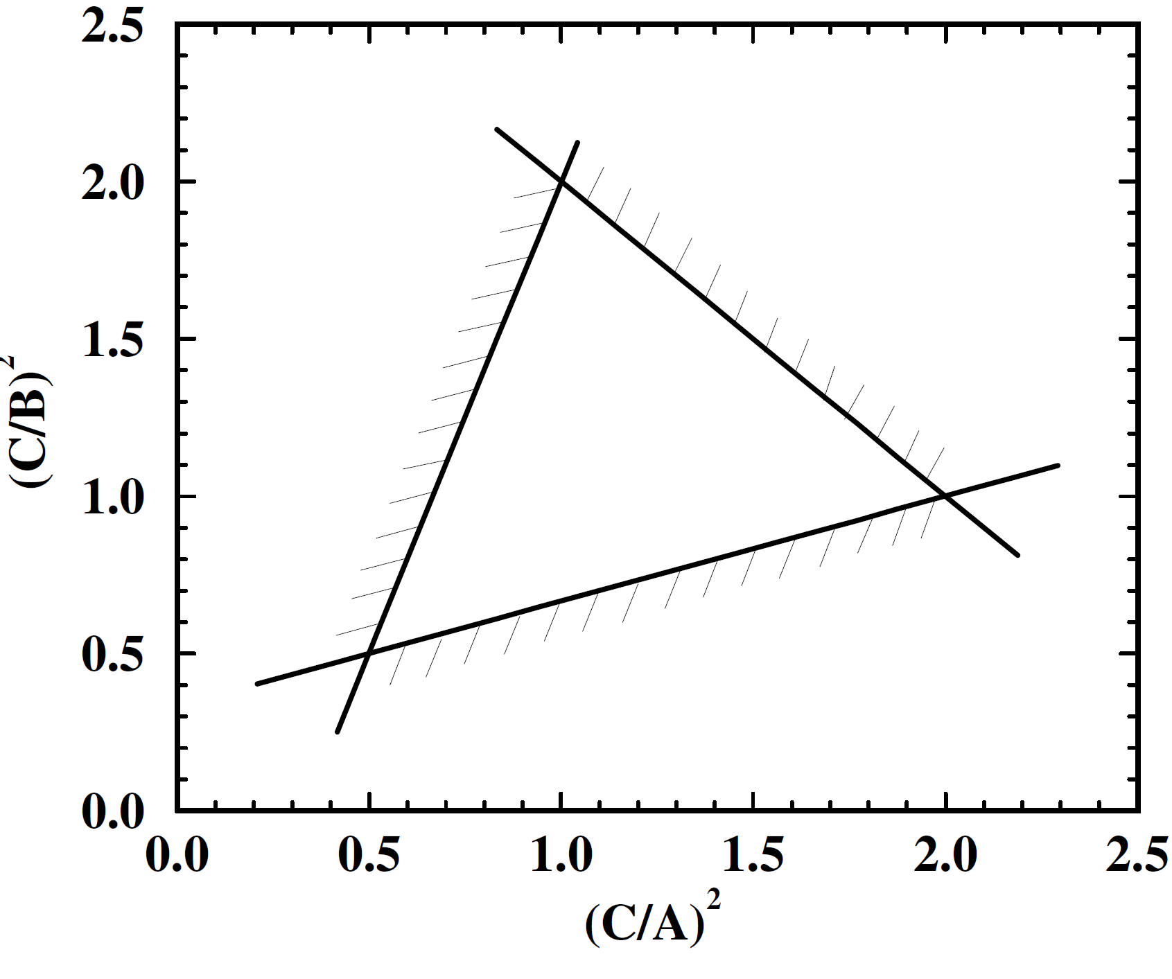
Fig. 3.46 Limits of Edge-Length Ratio for Positive Coefficients in 3D CVFEM.
The integration points in the CVFEM scheme can be shifted by
, , and  in the , , and directions.
The conditions for positive coefficients are
in the , , and directions.
The conditions for positive coefficients are
(3.1173)
(3.1174)
(3.1175)
The relations are nonlinear and require iteration to extract
the limiting values of , , and .
The coefficients that are generated by the standard GFEM operator in three dimensions have no allowable maximum aspect ratio. The only element shape that does not have negative coefficients is a cube, and even then the coefficients of the six nearest nodes are zero. The parametric representation of the nodal coefficients for the element contribution to the equation associated with Node 1 are
(3.1176)
(3.1177)
(3.1178)
(3.1179)
(3.1180)
(3.1181)
(3.1182)
(3.1183)
The contributions from Nodes 2, 4, and 5 are such that there will be negative coefficients for any element shape other than a cube.
Single-point integration is also used for the GFEM hexahedral element. Unfortunately, there is not a clear analogy between the integration point shift and hour-glass stabilization in three dimensions. The element matrix for the hour-glass stabilization term is
(3.1184)![\!\!\!C_{\rm hg} \!\left[\!
\begin{array}{rrrrrrrr}
-4\! 2\! 0\! 2\! 2\! 0\! -2\! 0\! \\
2\! -4\! 2\! 0\! 0\! 2\! 0\! -2\! \\
0\! 2\! -4\! 2\! -2\! 0\! 2\! 0\! \\
2\! 0\! 2\! -4\! 0\! -2\! 0\! 2\! \\
2\! 0\! -2\! 0\! -4\! 2\! 0\! 2\! \\
0\! 2\! 0\! -2\! 2\! -4\! 2\! 0\! \\
-2\! 0\! 2\! 0\! 0\! 2\! -4\! 2\! \\
0\! -2\! 0\! 2\! 2\! 0\! 2\! -4\!
\end{array}
\right],](data:image/svg+xml;base64,PD94bWwgdmVyc2lvbj0nMS4wJyBlbmNvZGluZz0nVVRGLTgnPz4KPCEtLSBUaGlzIGZpbGUgd2FzIGdlbmVyYXRlZCBieSBkdmlzdmdtIDMuMC4zIC0tPgo8c3ZnIHZlcnNpb249JzEuMScgeG1sbnM9J2h0dHA6Ly93d3cudzMub3JnLzIwMDAvc3ZnJyB4bWxuczp4bGluaz0naHR0cDovL3d3dy53My5vcmcvMTk5OS94bGluaycgd2lkdGg9JzEyMy4xODkwNTlwdCcgaGVpZ2h0PScxMzMuODk5MjNwdCcgdmlld0JveD0nMTI5LjE5MDA1MiAtMTM0LjY5NTU2NCAxMjMuMTg5MDU5IDEzMy44OTkyMyc+CjxkZWZzPgo8cGF0aCBpZD0nZzEtMCcgZD0nTTkuMTkxNTMyLTMuMjA3OTdDOS40Mjg2NDMtMy4yMDc5NyA5LjY3OTcwMS0zLjIwNzk3IDkuNjc5NzAxLTMuNDg2OTI0UzkuNDI4NjQzLTMuNzY1ODc4IDkuMTkxNTMyLTMuNzY1ODc4SDEuNjQ1ODI4QzEuNDA4NzE3LTMuNzY1ODc4IDEuMTU3NjU5LTMuNzY1ODc4IDEuMTU3NjU5LTMuNDg2OTI0UzEuNDA4NzE3LTMuMjA3OTcgMS42NDU4MjgtMy4yMDc5N0g5LjE5MTUzMlonLz4KPHBhdGggaWQ9J2c0LTQ4JyBkPSdNNi4yNDg1NjgtNC40NjMyNjNDNi4yNDg1NjgtNS42MjA5MjIgNi4xNzg4MjktNi43NTA2ODUgNS42NzY3MTItNy44MTA3MUM1LjEwNDg1Ny04Ljk2ODM2OSA0LjEwMDYyMy05LjI3NTIxOCAzLjQxNzE4Ni05LjI3NTIxOEMyLjYwODIxOS05LjI3NTIxOCAxLjYxNzkzMy04Ljg3MDczNSAxLjEwMTg2OC03LjcxMzA3NkMuNzExMzMzLTYuODM0MzcxIC41NzE4NTYtNS45Njk2MTQgLjU3MTg1Ni00LjQ2MzI2M0MuNTcxODU2LTMuMTEwMzM2IC42Njk0ODktMi4wOTIxNTQgMS4xNzE2MDYtMS4xMDE4NjhDMS43MTU1NjctLjA0MTg0MyAyLjY3Nzk1OCAuMjkyOTAyIDMuNDAzMjM4IC4yOTI5MDJDNC42MTY2ODcgLjI5MjkwMiA1LjMxNDA3Mi0uNDMyMzc5IDUuNzE4NTU1LTEuMjQxMzQ1QzYuMjIwNjcyLTIuMjg3NDIyIDYuMjQ4NTY4LTMuNjU0Mjk2IDYuMjQ4NTY4LTQuNDYzMjYzWk0zLjQwMzIzOCAuMDEzOTQ4QzIuOTU2OTEyIC4wMTM5NDggMi4wNTAzMTEtLjIzNzExMSAxLjc4NTMwNS0xLjc1NzQxQzEuNjMxODgtMi41OTQyNzEgMS42MzE4OC0zLjY1NDI5NiAxLjYzMTg4LTQuNjMwNjM1QzEuNjMxODgtNS43NzQzNDYgMS42MzE4OC02LjgwNjQ3NiAxLjg1NTA0NC03LjYyOTM5QzIuMDkyMTU0LTguNTYzODg1IDIuODAzNDg3LTguOTk2MjY0IDMuNDAzMjM4LTguOTk2MjY0QzMuOTMzMjUtOC45OTYyNjQgNC43NDIyMTctOC42NzU0NjcgNS4wMDcyMjMtNy40NzU5NjVDNS4xODg1NDMtNi42ODA5NDYgNS4xODg1NDMtNS41NzkwNzggNS4xODg1NDMtNC42MzA2MzVDNS4xODg1NDMtMy42OTYxMzkgNS4xODg1NDMtMi42MzYxMTUgNS4wMzUxMTgtMS43ODUzMDVDNC43NzAxMTItLjI1MTA1OSAzLjg5MTQwNyAuMDEzOTQ4IDMuNDAzMjM4IC4wMTM5NDhaJy8+CjxwYXRoIGlkPSdnNC01MCcgZD0nTTYuMTM2OTg2LTIuMzQzMjEzSDUuODMwMTM3QzUuNzg4Mjk0LTIuMTA2MTAyIDUuNjc2NzEyLTEuMzM4OTc5IDUuNTM3MjM1LTEuMTE1ODE2QzUuNDM5NjAxLS45OTAyODYgNC42NDQ1ODMtLjk5MDI4NiA0LjIyNjE1Mi0uOTkwMjg2SDEuNjQ1ODI4QzIuMDIyNDE2LTEuMzExMDgzIDIuODczMjI1LTIuMjAzNzM2IDMuMjM1ODY2LTIuNTM4NDgxQzUuMzU1OTE1LTQuNDkxMTU4IDYuMTM2OTg2LTUuMjE2NDM4IDYuMTM2OTg2LTYuNTk3MjZDNi4xMzY5ODYtOC4yMDEyNDUgNC44Njc3NDYtOS4yNzUyMTggMy4yNDk4MTMtOS4yNzUyMThTLjY4MzQzNy03Ljg5NDM5NiAuNjgzNDM3LTYuNjk0ODk0Qy42ODM0MzctNS45ODM1NjIgMS4yOTcxMzYtNS45ODM1NjIgMS4zMzg5NzktNS45ODM1NjJDMS42MzE4OC01Ljk4MzU2MiAxLjk5NDUyMS02LjE5Mjc3NyAxLjk5NDUyMS02LjYzOTEwM0MxLjk5NDUyMS03LjAyOTYzOSAxLjcyOTUxNC03LjI5NDY0NSAxLjMzODk3OS03LjI5NDY0NUMxLjIxMzQ1LTcuMjk0NjQ1IDEuMTg1NTU0LTcuMjk0NjQ1IDEuMTQzNzExLTcuMjgwNjk3QzEuNDA4NzE3LTguMjI5MTQxIDIuMTYxODkzLTguODcwNzM1IDMuMDY4NDkzLTguODcwNzM1QzQuMjU0MDQ3LTguODcwNzM1IDQuOTc5MzI4LTcuODgwNDQ4IDQuOTc5MzI4LTYuNTk3MjZDNC45NzkzMjgtNS40MTE3MDYgNC4yOTU4OS00LjM3OTU3NyAzLjUwMDg3Mi0zLjQ4NjkyNEwuNjgzNDM3LS4zMzQ3NDVWMEg1Ljc3NDM0Nkw2LjEzNjk4Ni0yLjM0MzIxM1onLz4KPHBhdGggaWQ9J2c0LTUyJyBkPSdNNS4wMzUxMTgtOS4wNzk5NUM1LjAzNTExOC05LjM0NDk1NiA1LjAzNTExOC05LjQxNDY5NSA0LjgzOTg1MS05LjQxNDY5NUM0LjcyODI2OS05LjQxNDY5NSA0LjY4NjQyNi05LjQxNDY5NSA0LjU3NDg0NC05LjI0NzMyM0wuMzc2NTg4LTIuNzMzNzQ4Vi0yLjMyOTI2NUg0LjA0NDgzMlYtMS4wNjAwMjVDNC4wNDQ4MzItLjU0Mzk2IDQuMDE2OTM2LS40MDQ0ODMgMi45OTg3NTUtLjQwNDQ4M0gyLjcxOTgwMVYwQzMuMDQwNTk4LS4wMjc4OTUgNC4xNDI0NjYtLjAyNzg5NSA0LjUzMzAwMS0uMDI3ODk1UzYuMDM5MzUyLS4wMjc4OTUgNi4zNjAxNDkgMFYtLjQwNDQ4M0g2LjA4MTE5NkM1LjA3Njk2MS0uNDA0NDgzIDUuMDM1MTE4LS41NDM5NiA1LjAzNTExOC0xLjA2MDAyNVYtMi4zMjkyNjVINi40NDM4MzZWLTIuNzMzNzQ4SDUuMDM1MTE4Vi05LjA3OTk1Wk00LjExNDU3LTcuOTkyMDNWLTIuNzMzNzQ4SC43MjUyOEw0LjExNDU3LTcuOTkyMDNaJy8+CjxwYXRoIGlkPSdnMC01MCcgZD0nTTQuNTQ2OTQ5IDI0LjU0Nzk0NUg1LjUwOTM0Vi40MTg0MzFIOS4xOTE1MzJWLS41NDM5Nkg0LjU0Njk0OVYyNC41NDc5NDVaJy8+CjxwYXRoIGlkPSdnMC01MScgZD0nTTMuNzc5ODI2IDI0LjU0Nzk0NUg0Ljc0MjIxN1YtLjU0Mzk2SC4wOTc2MzRWLjQxODQzMUgzLjc3OTgyNlYyNC41NDc5NDVaJy8+CjxwYXRoIGlkPSdnMC01MicgZD0nTTQuNTQ2OTQ5IDI0LjUzMzk5OEg5LjE5MTUzMlYyMy41NzE2MDZINS41MDkzNFYtLjU1NzkwOEg0LjU0Njk0OVYyNC41MzM5OThaJy8+CjxwYXRoIGlkPSdnMC01MycgZD0nTTMuNzc5ODI2IDIzLjU3MTYwNkguMDk3NjM0VjI0LjUzMzk5OEg0Ljc0MjIxN1YtLjU1NzkwOEgzLjc3OTgyNlYyMy41NzE2MDZaJy8+CjxwYXRoIGlkPSdnMC01NCcgZD0nTTQuNTQ2OTQ5IDguMzgyNTY1SDUuNTA5MzRWLS4wMTM5NDhINC41NDY5NDlWOC4zODI1NjVaJy8+CjxwYXRoIGlkPSdnMC01NScgZD0nTTMuNzc5ODI2IDguMzgyNTY1SDQuNzQyMjE3Vi0uMDEzOTQ4SDMuNzc5ODI2VjguMzgyNTY1WicvPgo8cGF0aCBpZD0nZzItNTknIGQ9J00yLjcxOTgwMSAuMDU1NzkxQzIuNzE5ODAxLS43NTMxNzYgMi40NTQ3OTUtMS4zNTI5MjcgMS44ODI5MzktMS4zNTI5MjdDMS40MzY2MTMtMS4zNTI5MjcgMS4yMTM0NS0uOTkwMjg2IDEuMjEzNDUtLjY4MzQzN1MxLjQyMjY2NSAwIDEuODk2ODg3IDBDMi4wNzgyMDcgMCAyLjIzMTYzMS0uMDU1NzkxIDIuMzU3MTYxLS4xODEzMkMyLjM4NTA1Ni0uMjA5MjE1IDIuMzk5MDA0LS4yMDkyMTUgMi40MTI5NTEtLjIwOTIxNUMyLjQ0MDg0Ny0uMjA5MjE1IDIuNDQwODQ3LS4wMTM5NDggMi40NDA4NDcgLjA1NTc5MUMyLjQ0MDg0NyAuNTE2MDY1IDIuMzU3MTYxIDEuNDIyNjY1IDEuNTQ4MTk0IDIuMzI5MjY1QzEuMzk0NzcgMi40OTY2MzggMS4zOTQ3NyAyLjUyNDUzMyAxLjM5NDc3IDIuNTUyNDI4QzEuMzk0NzcgMi42MjIxNjcgMS40NjQ1MDggMi42OTE5MDUgMS41MzQyNDcgMi42OTE5MDVDMS42NDU4MjggMi42OTE5MDUgMi43MTk4MDEgMS42NTk3NzYgMi43MTk4MDEgLjA1NTc5MVonLz4KPHBhdGggaWQ9J2cyLTY3JyBkPSdNMTAuNDE4OTI5LTkuNjkzNjQ5QzEwLjQxODkyOS05LjgxOTE3OCAxMC4zMjEyOTUtOS44MTkxNzggMTAuMjkzNC05LjgxOTE3OFMxMC4yMDk3MTQtOS44MTkxNzggMTAuMDk4MTMyLTkuNjc5NzAxTDkuMTM1NzQxLTguNTA4MDk1QzguNjQ3NTcyLTkuMzQ0OTU2IDcuODgwNDQ4LTkuODE5MTc4IDYuODM0MzcxLTkuODE5MTc4QzMuODIxNjY5LTkuODE5MTc4IC42OTczODUtNi43NjQ2MzMgLjY5NzM4NS0zLjQ4NjkyNEMuNjk3Mzg1LTEuMTU3NjU5IDIuMzI5MjY1IC4yOTI5MDIgNC4zNjU2MjkgLjI5MjkwMkM1LjQ4MTQ0NSAuMjkyOTAyIDYuNDU3NzgzLS4xODEzMiA3LjI2Njc1LS44NjQ3NTdDOC40ODAxOTktMS44ODI5MzkgOC44NDI4MzktMy4yMzU4NjYgOC44NDI4MzktMy4zNDc0NDdDOC44NDI4MzktMy40NzI5NzYgOC43MzEyNTgtMy40NzI5NzYgOC42ODk0MTUtMy40NzI5NzZDOC41NjM4ODUtMy40NzI5NzYgOC41NDk5MzgtMy4zODkyOSA4LjUyMjA0Mi0zLjMzMzQ5OUM3Ljg4MDQ0OC0xLjE1NzY1OSA1Ljk5NzUwOS0uMTExNTgyIDQuNjAyNzQtLjExMTU4MkMzLjEyNDI4NC0uMTExNTgyIDEuODQxMDk2LTEuMDYwMDI1IDEuODQxMDk2LTMuMDQwNTk4QzEuODQxMDk2LTMuNDg2OTI0IDEuOTgwNTczLTUuOTEzODIzIDMuNTU2NjYzLTcuNzQwOTcxQzQuMzIzNzg2LTguNjMzNjI0IDUuNjM0ODY5LTkuNDE0Njk1IDYuOTU5OS05LjQxNDY5NUM4LjQ5NDE0Ny05LjQxNDY5NSA5LjE3NzU4NC04LjE0NTQ1NSA5LjE3NzU4NC02LjcyMjc5QzkuMTc3NTg0LTYuMzYwMTQ5IDkuMTM1NzQxLTYuMDUzMyA5LjEzNTc0MS01Ljk5NzUwOUM5LjEzNTc0MS01Ljg3MTk4IDkuMjc1MjE4LTUuODcxOTggOS4zMTcwNjEtNS44NzE5OEM5LjQ3MDQ4Ni01Ljg3MTk4IDkuNDg0NDMzLTUuODg1OTI4IDkuNTQwMjI0LTYuMTM2OTg2TDEwLjQxODkyOS05LjY5MzY0OVonLz4KPHBhdGggaWQ9J2czLTEwMycgZD0nTTIuMTY3NDYzLTEuNjc5Mjk1QzEuMzE4MDUyLTEuNjc5Mjk1IDEuMzE4MDUyLTIuNjU1NjMgMS4zMTgwNTItMi44ODAxODdDMS4zMTgwNTItMy4xNDM3OTcgMS4zMjc4MTUtMy40NTYyMjQgMS40NzQyNjUtMy43MDAzMDhDMS41NTIzNzItMy44MTc0NjggMS43NzY5MjktNC4wOTA4NDEgMi4xNjc0NjMtNC4wOTA4NDFDMy4wMTY4NzQtNC4wOTA4NDEgMy4wMTY4NzQtMy4xMTQ1MDcgMy4wMTY4NzQtMi44ODk5NUMzLjAxNjg3NC0yLjYyNjM0IDMuMDA3MTEtMi4zMTM5MTMgMi44NjA2Ni0yLjA2OTgyOUMyLjc4MjU1My0xLjk1MjY2OSAyLjU1Nzk5Ni0xLjY3OTI5NSAyLjE2NzQ2My0xLjY3OTI5NVpNMS4wMzQ5MTUtMS4yOTg1MjVDMS4wMzQ5MTUtMS4zMzc1NzggMS4wMzQ5MTUtMS41NjIxMzUgMS4yMDA4OTEtMS43NTc0MDJDMS41ODE2NjItMS40ODQwMjggMS45ODE5NTktMS40NTQ3MzggMi4xNjc0NjMtMS40NTQ3MzhDMy4wNzU0NTQtMS40NTQ3MzggMy43NDkxMjQtMi4xMjg0MDkgMy43NDkxMjQtMi44ODAxODdDMy43NDkxMjQtMy4yNDE0MyAzLjU5MjkxMS0zLjYwMjY3NCAzLjM0ODgyNy0zLjgyNzIzMUMzLjcwMDMwOC00LjE1OTE4NSA0LjA1MTc4OC00LjIwODAwMiA0LjIyNzUyOC00LjIwODAwMkM0LjI0NzA1NS00LjIwODAwMiA0LjI5NTg3Mi00LjIwODAwMiA0LjMyNTE2Mi00LjE5ODIzOEM0LjIxNzc2NS00LjE1OTE4NSA0LjE2ODk0OC00LjA1MTc4OCA0LjE2ODk0OC0zLjkzNDYyOEM0LjE2ODk0OC0zLjc2ODY1MSA0LjI5NTg3Mi0zLjY1MTQ5MSA0LjQ1MjA4NS0zLjY1MTQ5MUM0LjU0OTcxOS0zLjY1MTQ5MSA0LjczNTIyMi0zLjcxOTgzNCA0LjczNTIyMi0zLjk0NDM5MUM0LjczNTIyMi00LjExMDM2OCA0LjYxODA2Mi00LjQyMjc5NSA0LjIzNzI5Mi00LjQyMjc5NUM0LjA0MjAyNS00LjQyMjc5NSAzLjYxMjQzOC00LjM2NDIxNSAzLjIwMjM3Ny0zLjk2MzkxOEMyLjc5MjMxNy00LjI4NjEwOCAyLjM4MjI1Ni00LjMxNTM5OCAyLjE2NzQ2My00LjMxNTM5OEMxLjI1OTQ3MS00LjMxNTM5OCAuNTg1ODAxLTMuNjQxNzI4IC41ODU4MDEtMi44ODk5NUMuNTg1ODAxLTIuNDYwMzYzIC44MDA1OTQtMi4wODkzNTYgMS4wNDQ2NzgtMS44ODQzMjZDLjkxNzc1NC0xLjczNzg3NSAuNzQyMDE0LTEuNDE1Njg1IC43NDIwMTQtMS4wNzM5NjhDLjc0MjAxNC0uNzcxMzA0IC44Njg5MzgtLjQwMDI5NyAxLjE3MTYwMS0uMjA1MDNDLjU4NTgwMS0uMDM5MDUzIC4yNzMzNzQgLjM4MDc3IC4yNzMzNzQgLjc3MTMwNEMuMjczMzc0IDEuNDc0MjY1IDEuMjM5OTQ1IDIuMDExMjQ5IDIuNDMxMDczIDIuMDExMjQ5QzMuNTgzMTQ4IDIuMDExMjQ5IDQuNTk4NTM1IDEuNTEzMzE4IDQuNTk4NTM1IC43NTE3NzhDNC41OTg1MzUgLjQxMDA2IDQuNDYxODQ5LS4wODc4NyAzLjk2MzkxOC0uMzYxMjQ0QzMuNDQ2NDYxLS42MzQ2MTcgMi44ODAxODctLjYzNDYxNyAyLjI4NDYyMy0uNjM0NjE3QzIuMDQwNTM5LS42MzQ2MTcgMS42MjA3MTUtLjYzNDYxNyAxLjU1MjM3Mi0uNjQ0MzgxQzEuMjM5OTQ1LS42ODM0MzQgMS4wMzQ5MTUtLjk4NjA5OCAxLjAzNDkxNS0xLjI5ODUyNVpNMi40NDA4MzYgMS43ODY2OTJDMS40NTQ3MzggMS43ODY2OTIgLjc4MTA2OCAxLjI4ODc2MiAuNzgxMDY4IC43NzEzMDRDLjc4MTA2OCAuMzIyMTkgMS4xNTIwNzUtLjAzOTA1MyAxLjU4MTY2Mi0uMDY4MzQzSDIuMTU3Njk5QzIuOTk3MzQ3LS4wNjgzNDMgNC4wOTA4NDEtLjA2ODM0MyA0LjA5MDg0MSAuNzcxMzA0QzQuMDkwODQxIDEuMjk4NTI1IDMuMzk3NjQ0IDEuNzg2NjkyIDIuNDQwODM2IDEuNzg2NjkyWicvPgo8cGF0aCBpZD0nZzMtMTA0JyBkPSdNMS4wNzM5NjgtLjc0MjAxNEMxLjA3Mzk2OC0uMzAyNjY0IC45NjY1NzEtLjMwMjY2NCAuMzEyNDI3LS4zMDI2NjRWMEMuNjU0MTQ0LS4wMDk3NjMgMS4xNTIwNzUtLjAyOTI5IDEuNDE1Njg1LS4wMjkyOUMxLjY2OTUzMi0uMDI5MjkgMi4xNzcyMjYtLjAwOTc2MyAyLjUwOTE4IDBWLS4zMDI2NjRDMS44NTUwMzUtLjMwMjY2NCAxLjc0NzYzOS0uMzAyNjY0IDEuNzQ3NjM5LS43NDIwMTRWLTIuNTM4NDdDMS43NDc2MzktMy41NTM4NTcgMi40NDA4MzYtNC4xMDA2MDUgMy4wNjU2OS00LjEwMDYwNUMzLjY4MDc4MS00LjEwMDYwNSAzLjc4ODE3OC0zLjU3MzM4NCAzLjc4ODE3OC0zLjAxNjg3NFYtLjc0MjAxNEMzLjc4ODE3OC0uMzAyNjY0IDMuNjgwNzgxLS4zMDI2NjQgMy4wMjY2MzctLjMwMjY2NFYwQzMuMzY4MzU0LS4wMDk3NjMgMy44NjYyODUtLjAyOTI5IDQuMTI5ODk1LS4wMjkyOUM0LjM4Mzc0Mi0uMDI5MjkgNC44OTE0MzYtLjAwOTc2MyA1LjIyMzM4OSAwVi0uMzAyNjY0QzQuNzE1Njk2LS4zMDI2NjQgNC40NzE2MTItLjMwMjY2NCA0LjQ2MTg0OS0uNTk1NTY0Vi0yLjQ2MDM2M0M0LjQ2MTg0OS0zLjMwMDAxMSA0LjQ2MTg0OS0zLjYwMjY3NCA0LjE1OTE4NS0zLjk1NDE1NUM0LjAyMjQ5OC00LjEyMDEzMSAzLjcwMDMwOC00LjMxNTM5OCAzLjEzNDAzNC00LjMxNTM5OEMyLjMxMzkxMy00LjMxNTM5OCAxLjg4NDMyNi0zLjcyOTU5OCAxLjcxODM0OS0zLjM1ODU5MVYtNi43NzU3NjFMLjMxMjQyNy02LjY2ODM2NFYtNi4zNjU3MDFDLjk5NTg2MS02LjM2NTcwMSAxLjA3Mzk2OC02LjI5NzM1NyAxLjA3Mzk2OC01LjgxODk1M1YtLjc0MjAxNFonLz4KPC9kZWZzPgo8ZyBpZD0ncGFnZTEnPgo8dXNlIHg9JzEyOS4xOTAwNTInIHk9Jy02NC4yNTkwMjknIHhsaW5rOmhyZWY9JyNnMi02NycvPgo8dXNlIHg9JzEzOC45NjA5MzknIHk9Jy02Mi4xNjY4ODMnIHhsaW5rOmhyZWY9JyNnMy0xMDQnLz4KPHVzZSB4PScxNDQuMzg1MDM2JyB5PSctNjIuMTY2ODgzJyB4bGluazpocmVmPScjZzMtMTAzJy8+Cjx1c2UgeD0nMTQ5LjkwMDQzJyB5PSctMTM0LjEzNzY3JyB4bGluazpocmVmPScjZzAtNTAnLz4KPHVzZSB4PScxNDkuOTAwNDMnIHk9Jy0xMDkuNTg5NDY3JyB4bGluazpocmVmPScjZzAtNTQnLz4KPHVzZSB4PScxNDkuOTAwNDMnIHk9Jy0xMDEuMjIwNzY0JyB4bGluazpocmVmPScjZzAtNTQnLz4KPHVzZSB4PScxNDkuOTAwNDMnIHk9Jy05Mi44NTIwNjEnIHhsaW5rOmhyZWY9JyNnMC01NCcvPgo8dXNlIHg9JzE0OS45MDA0MycgeT0nLTg0LjQ4MzM1OCcgeGxpbms6aHJlZj0nI2cwLTU0Jy8+Cjx1c2UgeD0nMTQ5LjkwMDQzJyB5PSctNzYuMTE0NjU1JyB4bGluazpocmVmPScjZzAtNTQnLz4KPHVzZSB4PScxNDkuOTAwNDMnIHk9Jy02Ny43NDU5NTMnIHhsaW5rOmhyZWY9JyNnMC01NCcvPgo8dXNlIHg9JzE0OS45MDA0MycgeT0nLTU5LjM3NzI1JyB4bGluazpocmVmPScjZzAtNTQnLz4KPHVzZSB4PScxNDkuOTAwNDMnIHk9Jy01MS4wMDg1NDcnIHhsaW5rOmhyZWY9JyNnMC01NCcvPgo8dXNlIHg9JzE0OS45MDA0MycgeT0nLTQyLjYzOTg0NCcgeGxpbms6aHJlZj0nI2cwLTU0Jy8+Cjx1c2UgeD0nMTQ5LjkwMDQzJyB5PSctMzQuMjcxMTQxJyB4bGluazpocmVmPScjZzAtNTQnLz4KPHVzZSB4PScxNDkuOTAwNDMnIHk9Jy0yNS4zNDQ1NDgnIHhsaW5rOmhyZWY9JyNnMC01MicvPgo8dXNlIHg9JzE2OC4wNTQ1NjYnIHk9Jy0xMjMuNjM2NDE1JyB4bGluazpocmVmPScjZzEtMCcvPgo8dXNlIHg9JzE3OC45MDI4MTInIHk9Jy0xMjMuNjM2NDE1JyB4bGluazpocmVmPScjZzQtNTInLz4KPHVzZSB4PScxODMuNDA2NzA1JyB5PSctMTIzLjYzNjQxNScgeGxpbms6aHJlZj0nI2c0LTUwJy8+Cjx1c2UgeD0nMTg3LjkxMDU5OCcgeT0nLTEyMy42MzY0MTUnIHhsaW5rOmhyZWY9JyNnNC00OCcvPgo8dXNlIHg9JzE5Mi40MTQ0OTEnIHk9Jy0xMjMuNjM2NDE1JyB4bGluazpocmVmPScjZzQtNTAnLz4KPHVzZSB4PScxOTYuOTE4Mzg0JyB5PSctMTIzLjYzNjQxNScgeGxpbms6aHJlZj0nI2c0LTUwJy8+Cjx1c2UgeD0nMjAxLjQyMjI3NycgeT0nLTEyMy42MzY0MTUnIHhsaW5rOmhyZWY9JyNnNC00OCcvPgo8dXNlIHg9JzIwOS4wMjU2MzEnIHk9Jy0xMjMuNjM2NDE1JyB4bGluazpocmVmPScjZzEtMCcvPgo8dXNlIHg9JzIyMi45NzMzMzgnIHk9Jy0xMjMuNjM2NDE1JyB4bGluazpocmVmPScjZzQtNTAnLz4KPHVzZSB4PScyMjcuNDc3MjMxJyB5PSctMTIzLjYzNjQxNScgeGxpbms6aHJlZj0nI2c0LTQ4Jy8+Cjx1c2UgeD0nMTYxLjg1NTY0NCcgeT0nLTEwNi42OTk5MjcnIHhsaW5rOmhyZWY9JyNnNC01MCcvPgo8dXNlIHg9JzE2OS40NTg5OTgnIHk9Jy0xMDYuNjk5OTI3JyB4bGluazpocmVmPScjZzEtMCcvPgo8dXNlIHg9JzE4My40MDY3MDUnIHk9Jy0xMDYuNjk5OTI3JyB4bGluazpocmVmPScjZzQtNTInLz4KPHVzZSB4PScxODcuOTEwNTk4JyB5PSctMTA2LjY5OTkyNycgeGxpbms6aHJlZj0nI2c0LTUwJy8+Cjx1c2UgeD0nMTkyLjQxNDQ5MScgeT0nLTEwNi42OTk5MjcnIHhsaW5rOmhyZWY9JyNnNC00OCcvPgo8dXNlIHg9JzE5Ni45MTgzODQnIHk9Jy0xMDYuNjk5OTI3JyB4bGluazpocmVmPScjZzQtNDgnLz4KPHVzZSB4PScyMDEuNDIyMjc3JyB5PSctMTA2LjY5OTkyNycgeGxpbms6aHJlZj0nI2c0LTUwJy8+Cjx1c2UgeD0nMjA1LjkyNjE3JyB5PSctMTA2LjY5OTkyNycgeGxpbms6aHJlZj0nI2c0LTQ4Jy8+Cjx1c2UgeD0nMjEzLjUyOTUyNCcgeT0nLTEwNi42OTk5MjcnIHhsaW5rOmhyZWY9JyNnMS0wJy8+Cjx1c2UgeD0nMjI3LjQ3NzIzMScgeT0nLTEwNi42OTk5MjcnIHhsaW5rOmhyZWY9JyNnNC01MCcvPgo8dXNlIHg9JzE2MS44NTU2NDQnIHk9Jy04OS43NjM0MzknIHhsaW5rOmhyZWY9JyNnNC00OCcvPgo8dXNlIHg9JzE2Ni4zNTk1MzcnIHk9Jy04OS43NjM0MzknIHhsaW5rOmhyZWY9JyNnNC01MCcvPgo8dXNlIHg9JzE3My45NjI4OTEnIHk9Jy04OS43NjM0MzknIHhsaW5rOmhyZWY9JyNnMS0wJy8+Cjx1c2UgeD0nMTg3LjkxMDU5OCcgeT0nLTg5Ljc2MzQzOScgeGxpbms6aHJlZj0nI2c0LTUyJy8+Cjx1c2UgeD0nMTkyLjQxNDQ5MScgeT0nLTg5Ljc2MzQzOScgeGxpbms6aHJlZj0nI2c0LTUwJy8+Cjx1c2UgeD0nMjAwLjAxNzg0NScgeT0nLTg5Ljc2MzQzOScgeGxpbms6aHJlZj0nI2cxLTAnLz4KPHVzZSB4PScyMTMuOTY1NTUzJyB5PSctODkuNzYzNDM5JyB4bGluazpocmVmPScjZzQtNTAnLz4KPHVzZSB4PScyMTguNDY5NDQ1JyB5PSctODkuNzYzNDM5JyB4bGluazpocmVmPScjZzQtNDgnLz4KPHVzZSB4PScyMjIuOTczMzM4JyB5PSctODkuNzYzNDM5JyB4bGluazpocmVmPScjZzQtNTAnLz4KPHVzZSB4PScyMjcuNDc3MjMxJyB5PSctODkuNzYzNDM5JyB4bGluazpocmVmPScjZzQtNDgnLz4KPHVzZSB4PScxNjEuODU1NjQ0JyB5PSctNzIuODI2OTUxJyB4bGluazpocmVmPScjZzQtNTAnLz4KPHVzZSB4PScxNjYuMzU5NTM3JyB5PSctNzIuODI2OTUxJyB4bGluazpocmVmPScjZzQtNDgnLz4KPHVzZSB4PScxNzAuODYzNDMnIHk9Jy03Mi44MjY5NTEnIHhsaW5rOmhyZWY9JyNnNC01MCcvPgo8dXNlIHg9JzE3OC40NjY3ODQnIHk9Jy03Mi44MjY5NTEnIHhsaW5rOmhyZWY9JyNnMS0wJy8+Cjx1c2UgeD0nMTkyLjQxNDQ5MScgeT0nLTcyLjgyNjk1MScgeGxpbms6aHJlZj0nI2c0LTUyJy8+Cjx1c2UgeD0nMTk2LjkxODM4NCcgeT0nLTcyLjgyNjk1MScgeGxpbms6aHJlZj0nI2c0LTQ4Jy8+Cjx1c2UgeD0nMjA0LjUyMTczOCcgeT0nLTcyLjgyNjk1MScgeGxpbms6aHJlZj0nI2cxLTAnLz4KPHVzZSB4PScyMTguNDY5NDQ1JyB5PSctNzIuODI2OTUxJyB4bGluazpocmVmPScjZzQtNTAnLz4KPHVzZSB4PScyMjIuOTczMzM4JyB5PSctNzIuODI2OTUxJyB4bGluazpocmVmPScjZzQtNDgnLz4KPHVzZSB4PScyMjcuNDc3MjMxJyB5PSctNzIuODI2OTUxJyB4bGluazpocmVmPScjZzQtNTAnLz4KPHVzZSB4PScxNjEuODU1NjQ0JyB5PSctNTUuODkwNDYzJyB4bGluazpocmVmPScjZzQtNTAnLz4KPHVzZSB4PScxNjYuMzU5NTM3JyB5PSctNTUuODkwNDYzJyB4bGluazpocmVmPScjZzQtNDgnLz4KPHVzZSB4PScxNzMuOTYyODkxJyB5PSctNTUuODkwNDYzJyB4bGluazpocmVmPScjZzEtMCcvPgo8dXNlIHg9JzE4Ny45MTA1OTgnIHk9Jy01NS44OTA0NjMnIHhsaW5rOmhyZWY9JyNnNC01MCcvPgo8dXNlIHg9JzE5Mi40MTQ0OTEnIHk9Jy01NS44OTA0NjMnIHhsaW5rOmhyZWY9JyNnNC00OCcvPgo8dXNlIHg9JzIwMC4wMTc4NDUnIHk9Jy01NS44OTA0NjMnIHhsaW5rOmhyZWY9JyNnMS0wJy8+Cjx1c2UgeD0nMjEzLjk2NTU1MycgeT0nLTU1Ljg5MDQ2MycgeGxpbms6aHJlZj0nI2c0LTUyJy8+Cjx1c2UgeD0nMjE4LjQ2OTQ0NScgeT0nLTU1Ljg5MDQ2MycgeGxpbms6aHJlZj0nI2c0LTUwJy8+Cjx1c2UgeD0nMjIyLjk3MzMzOCcgeT0nLTU1Ljg5MDQ2MycgeGxpbms6aHJlZj0nI2c0LTQ4Jy8+Cjx1c2UgeD0nMjI3LjQ3NzIzMScgeT0nLTU1Ljg5MDQ2MycgeGxpbms6aHJlZj0nI2c0LTUwJy8+Cjx1c2UgeD0nMTYxLjg1NTY0NCcgeT0nLTM4Ljk1Mzk3NCcgeGxpbms6aHJlZj0nI2c0LTQ4Jy8+Cjx1c2UgeD0nMTY2LjM1OTUzNycgeT0nLTM4Ljk1Mzk3NCcgeGxpbms6aHJlZj0nI2c0LTUwJy8+Cjx1c2UgeD0nMTcwLjg2MzQzJyB5PSctMzguOTUzOTc0JyB4bGluazpocmVmPScjZzQtNDgnLz4KPHVzZSB4PScxNzguNDY2Nzg0JyB5PSctMzguOTUzOTc0JyB4bGluazpocmVmPScjZzEtMCcvPgo8dXNlIHg9JzE5Mi40MTQ0OTEnIHk9Jy0zOC45NTM5NzQnIHhsaW5rOmhyZWY9JyNnNC01MCcvPgo8dXNlIHg9JzE5Ni45MTgzODQnIHk9Jy0zOC45NTM5NzQnIHhsaW5rOmhyZWY9JyNnNC01MCcvPgo8dXNlIHg9JzIwNC41MjE3MzgnIHk9Jy0zOC45NTM5NzQnIHhsaW5rOmhyZWY9JyNnMS0wJy8+Cjx1c2UgeD0nMjE4LjQ2OTQ0NScgeT0nLTM4Ljk1Mzk3NCcgeGxpbms6aHJlZj0nI2c0LTUyJy8+Cjx1c2UgeD0nMjIyLjk3MzMzOCcgeT0nLTM4Ljk1Mzk3NCcgeGxpbms6aHJlZj0nI2c0LTUwJy8+Cjx1c2UgeD0nMjI3LjQ3NzIzMScgeT0nLTM4Ljk1Mzk3NCcgeGxpbms6aHJlZj0nI2c0LTQ4Jy8+Cjx1c2UgeD0nMTY4LjA1NDU2NicgeT0nLTIyLjAxNzQ4NicgeGxpbms6aHJlZj0nI2cxLTAnLz4KPHVzZSB4PScxNzguOTAyODEyJyB5PSctMjIuMDE3NDg2JyB4bGluazpocmVmPScjZzQtNTAnLz4KPHVzZSB4PScxODMuNDA2NzA1JyB5PSctMjIuMDE3NDg2JyB4bGluazpocmVmPScjZzQtNDgnLz4KPHVzZSB4PScxODcuOTEwNTk4JyB5PSctMjIuMDE3NDg2JyB4bGluazpocmVmPScjZzQtNTAnLz4KPHVzZSB4PScxOTIuNDE0NDkxJyB5PSctMjIuMDE3NDg2JyB4bGluazpocmVmPScjZzQtNDgnLz4KPHVzZSB4PScxOTYuOTE4Mzg0JyB5PSctMjIuMDE3NDg2JyB4bGluazpocmVmPScjZzQtNDgnLz4KPHVzZSB4PScyMDEuNDIyMjc3JyB5PSctMjIuMDE3NDg2JyB4bGluazpocmVmPScjZzQtNTAnLz4KPHVzZSB4PScyMDkuMDI1NjMxJyB5PSctMjIuMDE3NDg2JyB4bGluazpocmVmPScjZzEtMCcvPgo8dXNlIHg9JzIyMi45NzMzMzgnIHk9Jy0yMi4wMTc0ODYnIHhsaW5rOmhyZWY9JyNnNC01MicvPgo8dXNlIHg9JzIyNy40NzcyMzEnIHk9Jy0yMi4wMTc0ODYnIHhsaW5rOmhyZWY9JyNnNC01MCcvPgo8dXNlIHg9JzE2MS44NTU2NDQnIHk9Jy01LjA4MDk5OCcgeGxpbms6aHJlZj0nI2c0LTQ4Jy8+Cjx1c2UgeD0nMTY5LjQ1ODk5OCcgeT0nLTUuMDgwOTk4JyB4bGluazpocmVmPScjZzEtMCcvPgo8dXNlIHg9JzE4My40MDY3MDUnIHk9Jy01LjA4MDk5OCcgeGxpbms6aHJlZj0nI2c0LTUwJy8+Cjx1c2UgeD0nMTg3LjkxMDU5OCcgeT0nLTUuMDgwOTk4JyB4bGluazpocmVmPScjZzQtNDgnLz4KPHVzZSB4PScxOTIuNDE0NDkxJyB5PSctNS4wODA5OTgnIHhsaW5rOmhyZWY9JyNnNC01MCcvPgo8dXNlIHg9JzE5Ni45MTgzODQnIHk9Jy01LjA4MDk5OCcgeGxpbms6aHJlZj0nI2c0LTUwJy8+Cjx1c2UgeD0nMjAxLjQyMjI3NycgeT0nLTUuMDgwOTk4JyB4bGluazpocmVmPScjZzQtNDgnLz4KPHVzZSB4PScyMDUuOTI2MTcnIHk9Jy01LjA4MDk5OCcgeGxpbms6aHJlZj0nI2c0LTUwJy8+Cjx1c2UgeD0nMjEzLjUyOTUyNCcgeT0nLTUuMDgwOTk4JyB4bGluazpocmVmPScjZzEtMCcvPgo8dXNlIHg9JzIyNy40NzcyMzEnIHk9Jy01LjA4MDk5OCcgeGxpbms6aHJlZj0nI2c0LTUyJy8+Cjx1c2UgeD0nMjM2Ljk2MjQyMScgeT0nLTEzNC4xMzc2NycgeGxpbms6aHJlZj0nI2cwLTUxJy8+Cjx1c2UgeD0nMjM2Ljk2MjQyMScgeT0nLTEwOS41ODk0NjcnIHhsaW5rOmhyZWY9JyNnMC01NScvPgo8dXNlIHg9JzIzNi45NjI0MjEnIHk9Jy0xMDEuMjIwNzY0JyB4bGluazpocmVmPScjZzAtNTUnLz4KPHVzZSB4PScyMzYuOTYyNDIxJyB5PSctOTIuODUyMDYxJyB4bGluazpocmVmPScjZzAtNTUnLz4KPHVzZSB4PScyMzYuOTYyNDIxJyB5PSctODQuNDgzMzU4JyB4bGluazpocmVmPScjZzAtNTUnLz4KPHVzZSB4PScyMzYuOTYyNDIxJyB5PSctNzYuMTE0NjU1JyB4bGluazpocmVmPScjZzAtNTUnLz4KPHVzZSB4PScyMzYuOTYyNDIxJyB5PSctNjcuNzQ1OTUzJyB4bGluazpocmVmPScjZzAtNTUnLz4KPHVzZSB4PScyMzYuOTYyNDIxJyB5PSctNTkuMzc3MjUnIHhsaW5rOmhyZWY9JyNnMC01NScvPgo8dXNlIHg9JzIzNi45NjI0MjEnIHk9Jy01MS4wMDg1NDcnIHhsaW5rOmhyZWY9JyNnMC01NScvPgo8dXNlIHg9JzIzNi45NjI0MjEnIHk9Jy00Mi42Mzk4NDQnIHhsaW5rOmhyZWY9JyNnMC01NScvPgo8dXNlIHg9JzIzNi45NjI0MjEnIHk9Jy0zNC4yNzExNDEnIHhsaW5rOmhyZWY9JyNnMC01NScvPgo8dXNlIHg9JzIzNi45NjI0MjEnIHk9Jy0yNS4zNDQ1NDgnIHhsaW5rOmhyZWY9JyNnMC01MycvPgo8dXNlIHg9JzI0OC41ODU1MDYnIHk9Jy02NC4yNTkwMjknIHhsaW5rOmhyZWY9JyNnMi01OScvPgo8L2c+Cjwvc3ZnPgo8IS0tIERFUFRIPTAgLS0+)
where the constant contains scaling information.
The hour-glass stabilization matrix does act to
make the diagonal terms more negative, and the problematic
off-diagonal terms more positive.