3.3.7. Lagrangian Particle Capabilities
3.3.7.1. Lagrangian Particle Spray: Diameter Cutoffs
The Fuego Lagrangian particle spray capability has a feature which allows an upper (high) and lower (low) size (diameter) cutoff to be set for particles inserted with a specified distribution (normal, normal mass, etc.). For distribution types with infinite tails like the standard normal distribution, the particle spray can select particle sizes small enough that they do not appear in the application of interest or so large that the assumption of the dilute spray model, inherent to the Fuego Lagrangian particle implementation, is violated. In specific applications where particles experience energetic chemical reactions, such as propellant fires, particles below a certain size range react quickly and disappear without the need to resolve their dynamics. The diameter cutoff feature allows the analyst to use standard distribution types while avoiding undesired particle size ranges. When diameter cutoffs are used, the particle pdf is adjusted accordingly to account for the lack of contribution from particle sizes outside the cutoff limits. The adjusted particle pdf is:
(3.734)
where  is the original, uncutoff particle size pdf,
  is the new particle pdf including low (
 ) and high (
 ) particle size cutoffs, the integral is take on the original particle pdf with these limits, and
  is the heaviside step function. This treatment properly normalizes . Figure 3.21 illustrates this for the case of a normal distribution of particle diameters (
 ) with and without diameter cutoffs at
  and
and  . Figure 3.22 shows a section of a Fuego input deck utilizing the diameter cutoff functionality.
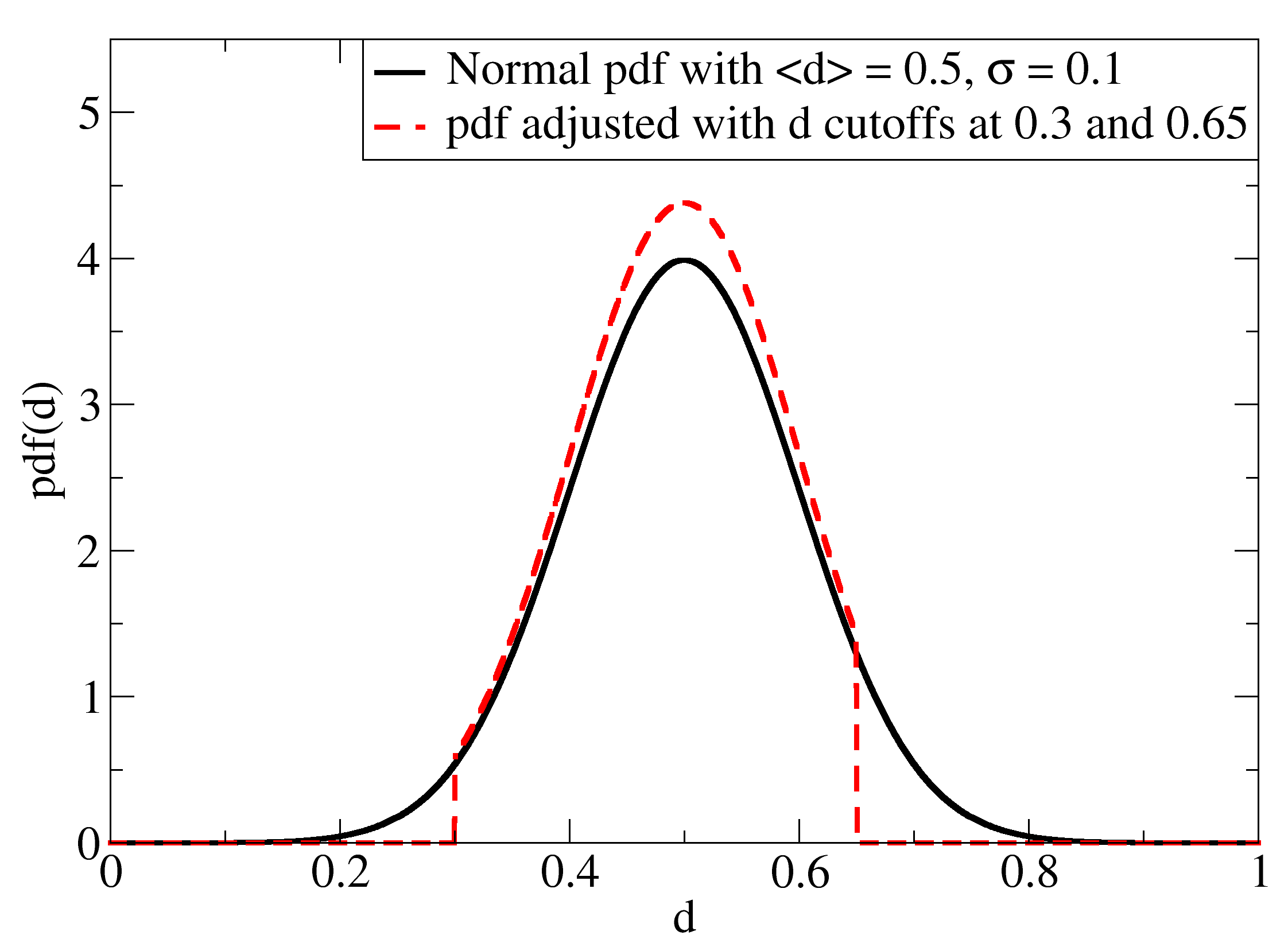
Fig. 3.21 Particle size (diameter) distribution for Lagrangian particle spray with and without diameter cutoffs set at  and
and 
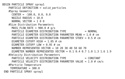
Fig. 3.22 Lagrangian particle spray section of a Fuego input deck showing use of diameter cutoffs
3.3.7.2. Lagrangian Particle Spray: Angular Spreading Sprays
The angular spreading spray algorithm was modified in version 4.30 to produce an isotropically spreading particle spray (within the angular limits specified). Previously, the particle trajectories were preferentially aligned with the spray axis. For isotropic spread, the cosine of the polar angle (measured with respect to the spray axis) rather than the angle itself is chosen randomly. The polar angle is then determined from the inverse cosine of this value.
(3.735)![\theta = cos^{-1}\left[rand\left(\right)\right]](data:image/svg+xml;base64,PD94bWwgdmVyc2lvbj0nMS4wJyBlbmNvZGluZz0nVVRGLTgnPz4KPCEtLSBUaGlzIGZpbGUgd2FzIGdlbmVyYXRlZCBieSBkdmlzdmdtIDMuMC4zIC0tPgo8c3ZnIHZlcnNpb249JzEuMScgeG1sbnM9J2h0dHA6Ly93d3cudzMub3JnLzIwMDAvc3ZnJyB4bWxuczp4bGluaz0naHR0cDovL3d3dy53My5vcmcvMTk5OS94bGluaycgd2lkdGg9JzEwOC43NzQxOTVwdCcgaGVpZ2h0PScxNS41Mzc3NDlwdCcgdmlld0JveD0nMTM5Ljg4NDQxNSAtMTcuMTMzODQ1IDEwOC43NzQxOTUgMTUuNTM3NzQ5Jz4KPGRlZnM+CjxwYXRoIGlkPSdnMi00OScgZD0nTTIuODcwNDIzLTYuMjQ4NTQxQzIuODcwNDIzLTYuNDgyODYxIDIuODcwNDIzLTYuNTAyMzg4IDIuNjQ1ODY2LTYuNTAyMzg4QzIuMDQwNTM5LTUuODc3NTM0IDEuMTgxMzY1LTUuODc3NTM0IC44Njg5MzgtNS44Nzc1MzRWLTUuNTc0ODdDMS4wNjQyMDUtNS41NzQ4NyAxLjY0MDI0Mi01LjU3NDg3IDIuMTQ3OTM2LTUuODI4NzE3Vi0uNzcxMzA0QzIuMTQ3OTM2LS40MTk4MjQgMi4xMTg2NDYtLjMwMjY2NCAxLjIzOTk0NS0uMzAyNjY0SC45Mjc1MThWMEMxLjI2OTIzNS0uMDI5MjkgMi4xMTg2NDYtLjAyOTI5IDIuNTA5MTgtLjAyOTI5UzMuNzQ5MTI0LS4wMjkyOSA0LjA5MDg0MSAwVi0uMzAyNjY0SDMuNzc4NDE0QzIuODk5NzEzLS4zMDI2NjQgMi44NzA0MjMtLjQxMDA2IDIuODcwNDIzLS43NzEzMDRWLTYuMjQ4NTQxWicvPgo8cGF0aCBpZD0nZzAtMCcgZD0nTTYuNDM0MDQ0LTIuMjQ1NTY5QzYuNjAwMDIxLTIuMjQ1NTY5IDYuNzc1NzYxLTIuMjQ1NTY5IDYuNzc1NzYxLTIuNDQwODM2UzYuNjAwMDIxLTIuNjM2MTAzIDYuNDM0MDQ0LTIuNjM2MTAzSDEuMTUyMDc1Qy45ODYwOTgtMi42MzYxMDMgLjgxMDM1OC0yLjYzNjEwMyAuODEwMzU4LTIuNDQwODM2Uy45ODYwOTgtMi4yNDU1NjkgMS4xNTIwNzUtMi4yNDU1NjlINi40MzQwNDRaJy8+CjxwYXRoIGlkPSdnMS0xOCcgZD0nTTYuMTc4ODI5LTcuMDE1NjkxQzYuMTc4ODI5LTguNDM4MzU2IDUuNzMyNTAzLTkuODE5MTc4IDQuNTg4NzkyLTkuODE5MTc4QzIuNjM2MTE1LTkuODE5MTc4IC41NTc5MDgtNS43MzI1MDMgLjU1NzkwOC0yLjY2NDAxQy41NTc5MDgtMi4wMjI0MTYgLjY5NzM4NSAuMTM5NDc3IDIuMTYxODkzIC4xMzk0NzdDNC4wNTg3OCAuMTM5NDc3IDYuMTc4ODI5LTMuODQ5NTY0IDYuMTc4ODI5LTcuMDE1NjkxWk0xLjk1MjY3Ny01LjA0OTA2NkMyLjE2MTg5My01Ljg3MTk4IDIuNDU0Nzk1LTcuMDQzNTg3IDMuMDEyNzAyLTguMDMzODczQzMuNDcyOTc2LTguODcwNzM1IDMuOTYxMTQ2LTkuNTQwMjI0IDQuNTc0ODQ0LTkuNTQwMjI0QzUuMDM1MTE4LTkuNTQwMjI0IDUuMzQxOTY4LTkuMTQ5Njg5IDUuMzQxOTY4LTcuODEwNzFDNS4zNDE5NjgtNy4zMDg1OTMgNS4zMDAxMjUtNi42MTEyMDggNC44OTU2NDEtNS4wNDkwNjZIMS45NTI2NzdaTTQuNzk4MDA3LTQuNjMwNjM1QzQuNDQ5MzE1LTMuMjYzNzYxIDQuMTU2NDEzLTIuMzg1MDU2IDMuNjU0Mjk2LTEuNTA2MzUxQzMuMjQ5ODEzLS43OTUwMTkgMi43NjE2NDQtLjEzOTQ3NyAyLjE3NTg0MS0uMTM5NDc3QzEuNzQzNDYyLS4xMzk0NzcgMS4zOTQ3Ny0uNDc0MjIyIDEuMzk0NzctMS44NTUwNDRDMS4zOTQ3Ny0yLjc2MTY0NCAxLjYxNzkzMy0zLjcxMDA4NyAxLjg0MTA5Ni00LjYzMDYzNUg0Ljc5ODAwN1onLz4KPHBhdGggaWQ9J2cxLTk3JyBkPSdNNC4xOTgyNTctMS42NTk3NzZDNC4xMjg1MTgtMS40MjI2NjUgNC4xMjg1MTgtMS4zOTQ3NyAzLjkzMzI1LTEuMTI5NzYzQzMuNjI2NDAxLS43MzkyMjggMy4wMTI3MDItLjEzOTQ3NyAyLjM1NzE2MS0uMTM5NDc3QzEuNzg1MzA1LS4xMzk0NzcgMS40NjQ1MDgtLjY1NTU0MiAxLjQ2NDUwOC0xLjQ3ODQ1NkMxLjQ2NDUwOC0yLjI0NTU3OSAxLjg5Njg4Ny0zLjgwNzcyMSAyLjE2MTg5My00LjM5MzUyNEMyLjYzNjExNS01LjM2OTg2MyAzLjI5MTY1Ni01Ljg3MTk4IDMuODM1NjE2LTUuODcxOThDNC43NTYxNjQtNS44NzE5OCA0LjkzNzQ4NC00LjcyODI2OSA0LjkzNzQ4NC00LjYxNjY4N0M0LjkzNzQ4NC00LjYwMjc0IDQuODk1NjQxLTQuNDIxNDIgNC44ODE2OTQtNC4zOTM1MjRMNC4xOTgyNTctMS42NTk3NzZaTTUuMDkwOTA5LTUuMjMwMzg2QzQuOTM3NDg0LTUuNTkzMDI2IDQuNTYwODk3LTYuMTUwOTM0IDMuODM1NjE2LTYuMTUwOTM0QzIuMjU5NTI3LTYuMTUwOTM0IC41NTc5MDgtNC4xMTQ1NyAuNTU3OTA4LTIuMDUwMzExQy41NTc5MDgtLjY2OTQ4OSAxLjM2Njg3NCAuMTM5NDc3IDIuMzE1MzE4IC4xMzk0NzdDMy4wODI0NDEgLjEzOTQ3NyAzLjczNzk4My0uNDYwMjc0IDQuMTI4NTE4LS45MjA1NDhDNC4yNjc5OTUtLjA5NzYzNCA0LjkyMzUzNyAuMTM5NDc3IDUuMzQxOTY4IC4xMzk0NzdTNi4wOTUxNDMtLjExMTU4MiA2LjM0NjIwMi0uNjEzNjk5QzYuNTY5MzY1LTEuMDg3OTIgNi43NjQ2MzMtMS45Mzg3MyA2Ljc2NDYzMy0xLjk5NDUyMUM2Ljc2NDYzMy0yLjA2NDI1OSA2LjcwODg0Mi0yLjEyMDA1IDYuNjI1MTU2LTIuMTIwMDVDNi40OTk2MjYtMi4xMjAwNSA2LjQ4NTY3OS0yLjA1MDMxMSA2LjQyOTg4OC0xLjg0MTA5NkM2LjIyMDY3Mi0xLjAxODE4MiA1Ljk1NTY2Ni0uMTM5NDc3IDUuMzgzODExLS4xMzk0NzdDNC45NzkzMjgtLjEzOTQ3NyA0Ljk1MTQzMi0uNTAyMTE3IDQuOTUxNDMyLS43ODEwNzFDNC45NTE0MzItMS4xMDE4NjggNC45OTMyNzUtMS4yNTUyOTMgNS4xMTg4MDQtMS43OTkyNTNDNS4yMTY0MzgtMi4xNDc5NDUgNS4yODYxNzctMi40NTQ3OTUgNS4zOTc3NTgtMi44NTkyNzhDNS45MTM4MjMtNC45NTE0MzIgNi4wMzkzNTItNS40NTM1NDkgNi4wMzkzNTItNS41MzcyMzVDNi4wMzkzNTItNS43MzI1MDMgNS44ODU5MjgtNS44ODU5MjggNS42NzY3MTItNS44ODU5MjhDNS4yMzAzODYtNS44ODU5MjggNS4xMTg4MDQtNS4zOTc3NTggNS4wOTA5MDktNS4yMzAzODZaJy8+CjxwYXRoIGlkPSdnMS05OScgZD0nTTUuNDUzNTQ5LTUuMjQ0MzM0QzUuMTg4NTQzLTUuMjQ0MzM0IDUuMDYzMDE0LTUuMjQ0MzM0IDQuODY3NzQ2LTUuMDc2OTYxQzQuNzg0MDYtNS4wMDcyMjMgNC42MzA2MzUtNC43OTgwMDcgNC42MzA2MzUtNC41NzQ4NDRDNC42MzA2MzUtNC4yOTU4OSA0LjgzOTg1MS00LjEyODUxOCA1LjEwNDg1Ny00LjEyODUxOEM1LjQzOTYwMS00LjEyODUxOCA1LjgxNjE4OS00LjQwNzQ3MiA1LjgxNjE4OS00Ljk2NTM4QzUuODE2MTg5LTUuNjM0ODY5IDUuMTc0NTk1LTYuMTUwOTM0IDQuMjEyMjA0LTYuMTUwOTM0QzIuMzg1MDU2LTYuMTUwOTM0IC41NTc5MDgtNC4xNTY0MTMgLjU1NzkwOC0yLjE3NTg0MUMuNTU3OTA4LS45NjIzOTEgMS4zMTEwODMgLjEzOTQ3NyAyLjczMzc0OCAuMTM5NDc3QzQuNjMwNjM1IC4xMzk0NzcgNS44MzAxMzctMS4zMzg5NzkgNS44MzAxMzctMS41MjAyOTlDNS44MzAxMzctMS42MDM5ODUgNS43NDY0NTEtMS42NzM3MjQgNS42OTA2Ni0xLjY3MzcyNEM1LjY0ODgxNy0xLjY3MzcyNCA1LjYzNDg2OS0xLjY1OTc3NiA1LjUwOTM0LTEuNTM0MjQ3QzQuNjE2Njg3LS4zNDg2OTIgMy4yOTE2NTYtLjEzOTQ3NyAyLjc2MTY0NC0uMTM5NDc3QzEuNzk5MjUzLS4xMzk0NzcgMS40OTI0MDMtLjk3NjMzOSAxLjQ5MjQwMy0xLjY3MzcyNEMxLjQ5MjQwMy0yLjE2MTg5MyAxLjcyOTUxNC0zLjUxNDgxOSAyLjIzMTYzMS00LjQ2MzI2M0MyLjU5NDI3MS01LjExODgwNCAzLjM0NzQ0Ny01Ljg3MTk4IDQuMjI2MTUyLTUuODcxOThDNC40MDc0NzItNS44NzE5OCA1LjE3NDU5NS01Ljg0NDA4NSA1LjQ1MzU0OS01LjI0NDMzNFonLz4KPHBhdGggaWQ9J2cxLTEwMCcgZD0nTTcuMDE1NjkxLTkuMzMxMDA5QzcuMDI5NjM5LTkuMzg2OCA3LjA1NzUzNC05LjQ3MDQ4NiA3LjA1NzUzNC05LjU0MDIyNEM3LjA1NzUzNC05LjY3OTcwMSA2LjkxODA1Ny05LjY3OTcwMSA2Ljg5MDE2Mi05LjY3OTcwMUM2Ljg3NjIxNC05LjY3OTcwMSA2LjE5Mjc3Ny05LjYyMzkxIDYuMTIzMDM5LTkuNjA5OTYzQzUuODg1OTI4LTkuNTk2MDE1IDUuNjc2NzEyLTkuNTY4MTIgNS40MjU2NTQtOS41NTQxNzJDNS4wNzY5NjEtOS41MjYyNzYgNC45NzkzMjgtOS41MTIzMjkgNC45NzkzMjgtOS4yNjEyN0M0Ljk3OTMyOC05LjEyMTc5MyA1LjA5MDkwOS05LjEyMTc5MyA1LjI4NjE3Ny05LjEyMTc5M0M1Ljk2OTYxNC05LjEyMTc5MyA1Ljk4MzU2Mi04Ljk5NjI2NCA1Ljk4MzU2Mi04Ljg1Njc4N0M1Ljk4MzU2Mi04Ljc3MzEwMSA1Ljk1NTY2Ni04LjY2MTUxOSA1Ljk0MTcxOS04LjYxOTY3Nkw1LjA5MDkwOS01LjIzMDM4NkM0LjkzNzQ4NC01LjU5MzAyNiA0LjU2MDg5Ny02LjE1MDkzNCAzLjgzNTYxNi02LjE1MDkzNEMyLjI1OTUyNy02LjE1MDkzNCAuNTU3OTA4LTQuMTE0NTcgLjU1NzkwOC0yLjA1MDMxMUMuNTU3OTA4LS42Njk0ODkgMS4zNjY4NzQgLjEzOTQ3NyAyLjMxNTMxOCAuMTM5NDc3QzMuMDgyNDQxIC4xMzk0NzcgMy43Mzc5ODMtLjQ2MDI3NCA0LjEyODUxOC0uOTIwNTQ4QzQuMjY3OTk1LS4wOTc2MzQgNC45MjM1MzcgLjEzOTQ3NyA1LjM0MTk2OCAuMTM5NDc3UzYuMDk1MTQzLS4xMTE1ODIgNi4zNDYyMDItLjYxMzY5OUM2LjU2OTM2NS0xLjA4NzkyIDYuNzY0NjMzLTEuOTM4NzMgNi43NjQ2MzMtMS45OTQ1MjFDNi43NjQ2MzMtMi4wNjQyNTkgNi43MDg4NDItMi4xMjAwNSA2LjYyNTE1Ni0yLjEyMDA1QzYuNDk5NjI2LTIuMTIwMDUgNi40ODU2NzktMi4wNTAzMTEgNi40Mjk4ODgtMS44NDEwOTZDNi4yMjA2NzItMS4wMTgxODIgNS45NTU2NjYtLjEzOTQ3NyA1LjM4MzgxMS0uMTM5NDc3QzQuOTc5MzI4LS4xMzk0NzcgNC45NTE0MzItLjUwMjExNyA0Ljk1MTQzMi0uNzgxMDcxQzQuOTUxNDMyLS44MzY4NjIgNC45NTE0MzItMS4xMjk3NjMgNS4wNDkwNjYtMS41MjAyOTlMNy4wMTU2OTEtOS4zMzEwMDlaTTQuMTk4MjU3LTEuNjU5Nzc2QzQuMTI4NTE4LTEuNDIyNjY1IDQuMTI4NTE4LTEuMzk0NzcgMy45MzMyNS0xLjEyOTc2M0MzLjYyNjQwMS0uNzM5MjI4IDMuMDEyNzAyLS4xMzk0NzcgMi4zNTcxNjEtLjEzOTQ3N0MxLjc4NTMwNS0uMTM5NDc3IDEuNDY0NTA4LS42NTU1NDIgMS40NjQ1MDgtMS40Nzg0NTZDMS40NjQ1MDgtMi4yNDU1NzkgMS44OTY4ODctMy44MDc3MjEgMi4xNjE4OTMtNC4zOTM1MjRDMi42MzYxMTUtNS4zNjk4NjMgMy4yOTE2NTYtNS44NzE5OCAzLjgzNTYxNi01Ljg3MTk4QzQuNzU2MTY0LTUuODcxOTggNC45Mzc0ODQtNC43MjgyNjkgNC45Mzc0ODQtNC42MTY2ODdDNC45Mzc0ODQtNC42MDI3NCA0Ljg5NTY0MS00LjQyMTQyIDQuODgxNjk0LTQuMzkzNTI0TDQuMTk4MjU3LTEuNjU5Nzc2WicvPgo8cGF0aCBpZD0nZzEtMTEwJyBkPSdNMi44NzMyMjUtNC4wODY2NzVDMi45MDExMjEtNC4xNzAzNjEgMy4yNDk4MTMtNC44Njc3NDYgMy43NjU4NzgtNS4zMTQwNzJDNC4xMjg1MTgtNS42NDg4MTcgNC42MDI3NC01Ljg3MTk4IDUuMTQ2Ny01Ljg3MTk4QzUuNzA0NjA4LTUuODcxOTggNS44OTk4NzUtNS40NTM1NDkgNS44OTk4NzUtNC44OTU2NDFDNS44OTk4NzUtNC4xMDA2MjMgNS4zMjgwMi0yLjUxMDU4NSA1LjA0OTA2Ni0xLjc1NzQxQzQuOTIzNTM3LTEuNDIyNjY1IDQuODUzNzk4LTEuMjQxMzQ1IDQuODUzNzk4LS45OTAyODZDNC44NTM3OTgtLjM2MjY0IDUuMjg2MTc3IC4xMzk0NzcgNS45NTU2NjYgLjEzOTQ3N0M3LjI1MjgwMiAuMTM5NDc3IDcuNzQwOTcxLTEuOTEwODM0IDcuNzQwOTcxLTEuOTk0NTIxQzcuNzQwOTcxLTIuMDY0MjU5IDcuNjg1MTgxLTIuMTIwMDUgNy42MDE0OTQtMi4xMjAwNUM3LjQ3NTk2NS0yLjEyMDA1IDcuNDYyMDE3LTIuMDc4MjA3IDcuMzkyMjc5LTEuODQxMDk2QzcuMDcxNDgyLS42OTczODUgNi41NDE0NjktLjEzOTQ3NyA1Ljk5NzUwOS0uMTM5NDc3QzUuODU4MDMyLS4xMzk0NzcgNS42MzQ4NjktLjE1MzQyNSA1LjYzNDg2OS0uNTk5NzUxQzUuNjM0ODY5LS45NDg0NDMgNS43ODgyOTQtMS4zNjY4NzQgNS44NzE5OC0xLjU2MjE0MkM2LjE1MDkzNC0yLjMyOTI2NSA2LjczNjczNy0zLjg5MTQwNyA2LjczNjczNy00LjY4NjQyNkM2LjczNjczNy01LjUyMzI4OCA2LjI0ODU2OC02LjE1MDkzNCA1LjE4ODU0My02LjE1MDkzNEMzLjk0NzE5OC02LjE1MDkzNCAzLjI5MTY1Ni01LjI3MjIyOSAzLjA0MDU5OC00LjkyMzUzN0MyLjk5ODc1NS01LjcxODU1NSAyLjQyNjg5OS02LjE1MDkzNCAxLjgxMzItNi4xNTA5MzRDMS4zNjY4NzQtNi4xNTA5MzQgMS4wNjAwMjUtNS44ODU5MjggLjgyMjkxNC01LjQxMTcwNkMuNTcxODU2LTQuOTA5NTg5IC4zNzY1ODgtNC4wNzI3MjcgLjM3NjU4OC00LjAxNjkzNlMuNDMyMzc5LTMuODkxNDA3IC41MzAwMTItMy44OTE0MDdDLjY0MTU5NC0zLjg5MTQwNyAuNjU1NTQyLTMuOTA1MzU1IC43MzkyMjgtNC4yMjYxNTJDLjk2MjM5MS01LjA3Njk2MSAxLjIxMzQ1LTUuODcxOTggMS43NzEzNTctNS44NzE5OEMyLjA5MjE1NC01Ljg3MTk4IDIuMjAzNzM2LTUuNjQ4ODE3IDIuMjAzNzM2LTUuMjMwMzg2QzIuMjAzNzM2LTQuOTIzNTM3IDIuMDY0MjU5LTQuMzc5NTc3IDEuOTY2NjI1LTMuOTQ3MTk4TDEuNTc2MDktMi40NDA4NDdDMS41MjAyOTktMi4xNzU4NDEgMS4zNjY4NzQtMS41NDgxOTQgMS4yOTcxMzYtMS4yOTcxMzZDMS4xOTk1MDItLjkzNDQ5NiAxLjA0NjA3Ny0uMjc4OTU0IDEuMDQ2MDc3LS4yMDkyMTVDMS4wNDYwNzctLjAxMzk0OCAxLjE5OTUwMiAuMTM5NDc3IDEuNDA4NzE3IC4xMzk0NzdDMS41NzYwOSAuMTM5NDc3IDEuNzcxMzU3IC4wNTU3OTEgMS44ODI5MzktLjE1MzQyNUMxLjkxMDgzNC0uMjIzMTYzIDIuMDM2MzY0LS43MTEzMzMgMi4xMDYxMDItLjk5MDI4NkwyLjQxMjk1MS0yLjI0NTU3OUwyLjg3MzIyNS00LjA4NjY3NVonLz4KPHBhdGggaWQ9J2cxLTExMScgZD0nTTYuMzYwMTQ5LTMuODM1NjE2QzYuMzYwMTQ5LTUuMTYwNjQ4IDUuNDk1MzkyLTYuMTUwOTM0IDQuMjI2MTUyLTYuMTUwOTM0QzIuMzg1MDU2LTYuMTUwOTM0IC41NzE4NTYtNC4xNDI0NjYgLjU3MTg1Ni0yLjE3NTg0MUMuNTcxODU2LS44NTA4MDkgMS40MzY2MTMgLjEzOTQ3NyAyLjcwNTg1MyAuMTM5NDc3QzQuNTYwODk3IC4xMzk0NzcgNi4zNjAxNDktMS44Njg5OTEgNi4zNjAxNDktMy44MzU2MTZaTTIuNzE5ODAxLS4xMzk0NzdDMi4wMjI0MTYtLjEzOTQ3NyAxLjUwNjM1MS0uNjk3Mzg1IDEuNTA2MzUxLTEuNjczNzI0QzEuNTA2MzUxLTIuMzE1MzE4IDEuODQxMDk2LTMuNzM3OTgzIDIuMjMxNjMxLTQuNDM1MzY3QzIuODU5Mjc4LTUuNTA5MzQgMy42NDAzNDktNS44NzE5OCA0LjIxMjIwNC01Ljg3MTk4QzQuODk1NjQxLTUuODcxOTggNS40MjU2NTQtNS4zMTQwNzIgNS40MjU2NTQtNC4zMzc3MzNDNS40MjU2NTQtMy43Nzk4MjYgNS4xMzI3NTItMi4yODc0MjIgNC42MDI3NC0xLjQzNjYxM0M0LjAzMDg4NC0uNTAyMTE3IDMuMjYzNzYxLS4xMzk0NzcgMi43MTk4MDEtLjEzOTQ3N1onLz4KPHBhdGggaWQ9J2cxLTExNCcgZD0nTTUuNDI1NjU0LTUuNzA0NjA4QzQuOTkzMjc1LTUuNjIwOTIyIDQuNzcwMTEyLTUuMzE0MDcyIDQuNzcwMTEyLTUuMDA3MjIzQzQuNzcwMTEyLTQuNjcyNDc4IDUuMDM1MTE4LTQuNTYwODk3IDUuMjMwMzg2LTQuNTYwODk3QzUuNjIwOTIyLTQuNTYwODk3IDUuOTQxNzE5LTQuODk1NjQxIDUuOTQxNzE5LTUuMzE0MDcyQzUuOTQxNzE5LTUuNzYwMzk5IDUuNTA5MzQtNi4xNTA5MzQgNC44MTE5NTUtNi4xNTA5MzRDNC4yNTQwNDctNi4xNTA5MzQgMy42MTI0NTMtNS44OTk4NzUgMy4wMjY2NS01LjA0OTA2NkMyLjkyOTAxNi01Ljc4ODI5NCAyLjM3MTEwOC02LjE1MDkzNCAxLjgxMzItNi4xNTA5MzRDMS4yNjkyNC02LjE1MDkzNCAuOTkwMjg2LTUuNzMyNTAzIC44MjI5MTQtNS40MjU2NTRDLjU4NTgwMy00LjkyMzUzNyAuMzc2NTg4LTQuMDg2Njc1IC4zNzY1ODgtNC4wMTY5MzZDLjM3NjU4OC0zLjk2MTE0NiAuNDMyMzc5LTMuODkxNDA3IC41MzAwMTItMy44OTE0MDdDLjY0MTU5NC0zLjg5MTQwNyAuNjU1NTQyLTMuOTA1MzU1IC43MzkyMjgtNC4yMjYxNTJDLjk0ODQ0My01LjA2MzAxNCAxLjIxMzQ1LTUuODcxOTggMS43NzEzNTctNS44NzE5OEMyLjEwNjEwMi01Ljg3MTk4IDIuMjAzNzM2LTUuNjM0ODY5IDIuMjAzNzM2LTUuMjMwMzg2QzIuMjAzNzM2LTQuOTIzNTM3IDIuMDY0MjU5LTQuMzc5NTc3IDEuOTY2NjI1LTMuOTQ3MTk4TDEuNTc2MDktMi40NDA4NDdDMS41MjAyOTktMi4xNzU4NDEgMS4zNjY4NzQtMS41NDgxOTQgMS4yOTcxMzYtMS4yOTcxMzZDMS4xOTk1MDItLjkzNDQ5NiAxLjA0NjA3Ny0uMjc4OTU0IDEuMDQ2MDc3LS4yMDkyMTVDMS4wNDYwNzctLjAxMzk0OCAxLjE5OTUwMiAuMTM5NDc3IDEuNDA4NzE3IC4xMzk0NzdDMS41NjIxNDIgLjEzOTQ3NyAxLjgyNzE0OCAuMDQxODQzIDEuOTEwODM0LS4yMzcxMTFDMS45NTI2NzctLjM0ODY5MiAyLjQ2ODc0Mi0yLjQ1NDc5NSAyLjU1MjQyOC0yLjc3NTU5MkMyLjYyMjE2Ny0zLjA4MjQ0MSAyLjcwNTg1My0zLjM3NTM0MiAyLjc3NTU5Mi0zLjY4MjE5MkMyLjgzMTM4Mi0zLjg3NzQ2IDIuODg3MTczLTQuMTAwNjIzIDIuOTI5MDE2LTQuMjgxOTQzQzIuOTcwODU5LTQuNDA3NDcyIDMuMzQ3NDQ3LTUuMDkwOTA5IDMuNjk2MTM5LTUuMzk3NzU4QzMuODYzNTEyLTUuNTUxMTgzIDQuMjI2MTUyLTUuODcxOTggNC43OTgwMDctNS44NzE5OEM1LjAyMTE3MS01Ljg3MTk4IDUuMjQ0MzM0LTUuODMwMTM3IDUuNDI1NjU0LTUuNzA0NjA4WicvPgo8cGF0aCBpZD0nZzEtMTE1JyBkPSdNMy4xODAwNzUtMi43ODk1MzlDMy40MTcxODYtMi43NDc2OTYgMy43OTM3NzMtMi42NjQwMSAzLjg3NzQ2LTIuNjUwMDYyQzQuMDU4NzgtMi41OTQyNzEgNC42ODY0MjYtMi4zNzExMDggNC42ODY0MjYtMS43MDE2MTlDNC42ODY0MjYtMS4yNjkyNCA0LjI5NTg5LS4xMzk0NzcgMi42Nzc5NTgtLjEzOTQ3N0MyLjM4NTA1Ni0uMTM5NDc3IDEuMzM4OTc5LS4xODEzMiAxLjA2MDAyNS0uOTQ4NDQzQzEuNjE3OTMzLS44Nzg3MDUgMS44OTY4ODctMS4zMTEwODMgMS44OTY4ODctMS42MTc5MzNDMS44OTY4ODctMS45MTA4MzQgMS43MDE2MTktMi4wNjQyNTkgMS40MjI2NjUtMi4wNjQyNTlDMS4xMTU4MTYtMi4wNjQyNTkgLjcxMTMzMy0xLjgyNzE0OCAuNzExMzMzLTEuMTk5NTAyQy43MTEzMzMtLjM3NjU4OCAxLjU0ODE5NCAuMTM5NDc3IDIuNjY0MDEgLjEzOTQ3N0M0Ljc4NDA2IC4xMzk0NzcgNS40MTE3MDYtMS40MjI2NjUgNS40MTE3MDYtMi4xNDc5NDVDNS40MTE3MDYtMi4zNTcxNjEgNS40MTE3MDYtMi43NDc2OTYgNC45NjUzOC0zLjE5NDAyMkM0LjYxNjY4Ny0zLjUyODc2NyA0LjI4MTk0My0zLjU5ODUwNiAzLjUyODc2Ny0zLjc1MTkzQzMuMTUyMTc5LTMuODM1NjE2IDIuNTUyNDI4LTMuOTYxMTQ2IDIuNTUyNDI4LTQuNTg4NzkyQzIuNTUyNDI4LTQuODY3NzQ2IDIuODAzNDg3LTUuODcxOTggNC4xMjg1MTgtNS44NzE5OEM0LjcxNDMyMS01Ljg3MTk4IDUuMjg2MTc3LTUuNjQ4ODE3IDUuNDI1NjU0LTUuMTQ2N0M0LjgxMTk1NS01LjE0NjcgNC43ODQwNi00LjYxNjY4NyA0Ljc4NDA2LTQuNjAyNzRDNC43ODQwNi00LjMwOTgzOCA1LjA0OTA2Ni00LjIyNjE1MiA1LjE3NDU5NS00LjIyNjE1MkM1LjM2OTg2My00LjIyNjE1MiA1Ljc2MDM5OS00LjM3OTU3NyA1Ljc2MDM5OS00Ljk2NTM4UzUuMjMwMzg2LTYuMTUwOTM0IDQuMTQyNDY2LTYuMTUwOTM0QzIuMzE1MzE4LTYuMTUwOTM0IDEuODI3MTQ4LTQuNzE0MzIxIDEuODI3MTQ4LTQuMTQyNDY2QzEuODI3MTQ4LTMuMDgyNDQxIDIuODU5Mjc4LTIuODU5Mjc4IDMuMTgwMDc1LTIuNzg5NTM5WicvPgo8cGF0aCBpZD0nZzMtNDAnIGQ9J000LjUzMzAwMSAzLjM4OTI5QzQuNTMzMDAxIDMuMzQ3NDQ3IDQuNTMzMDAxIDMuMzE5NTUyIDQuMjk1ODkgMy4wODI0NDFDMi45MDExMjEgMS42NzM3MjQgMi4xMjAwNS0uNjI3NjQ2IDIuMTIwMDUtMy40NzI5NzZDMi4xMjAwNS02LjE3ODgyOSAyLjc3NTU5Mi04LjUwODA5NSA0LjM5MzUyNC0xMC4xNTM5MjNDNC41MzMwMDEtMTAuMjc5NDUyIDQuNTMzMDAxLTEwLjMwNzM0NyA0LjUzMzAwMS0xMC4zNDkxOTFDNC41MzMwMDEtMTAuNDMyODc3IDQuNDYzMjYzLTEwLjQ2MDc3MiA0LjQwNzQ3Mi0xMC40NjA3NzJDNC4yMjYxNTItMTAuNDYwNzcyIDMuMDgyNDQxLTkuNDU2NTM4IDIuMzk5MDA0LTguMDg5NjY0QzEuNjg3NjcxLTYuNjgwOTQ2IDEuMzY2ODc0LTUuMTg4NTQzIDEuMzY2ODc0LTMuNDcyOTc2QzEuMzY2ODc0LTIuMjMxNjMxIDEuNTYyMTQyLS41NzE4NTYgMi4yODc0MjIgLjkyMDU0OEMzLjExMDMzNiAyLjU5NDI3MSA0LjI1NDA0NyAzLjUwMDg3MiA0LjQwNzQ3MiAzLjUwMDg3MkM0LjQ2MzI2MyAzLjUwMDg3MiA0LjUzMzAwMSAzLjQ3Mjk3NiA0LjUzMzAwMSAzLjM4OTI5WicvPgo8cGF0aCBpZD0nZzMtNDEnIGQ9J00zLjkzMzI1LTMuNDcyOTc2QzMuOTMzMjUtNC41MzMwMDEgMy43OTM3NzMtNi4yNjI1MTYgMy4wMTI3MDItNy44ODA0NDhDMi4xODk3ODgtOS41NTQxNzIgMS4wNDYwNzctMTAuNDYwNzcyIC44OTI2NTMtMTAuNDYwNzcyQy44MzY4NjItMTAuNDYwNzcyIC43NjcxMjMtMTAuNDMyODc3IC43NjcxMjMtMTAuMzQ5MTkxQy43NjcxMjMtMTAuMzA3MzQ3IC43NjcxMjMtMTAuMjc5NDUyIDEuMDA0MjM0LTEwLjA0MjM0MUMyLjM5OTAwNC04LjYzMzYyNCAzLjE4MDA3NS02LjMzMjI1NCAzLjE4MDA3NS0zLjQ4NjkyNEMzLjE4MDA3NS0uNzgxMDcxIDIuNTI0NTMzIDEuNTQ4MTk0IC45MDY2IDMuMTk0MDIyQy43NjcxMjMgMy4zMTk1NTIgLjc2NzEyMyAzLjM0NzQ0NyAuNzY3MTIzIDMuMzg5MjlDLjc2NzEyMyAzLjQ3Mjk3NiAuODM2ODYyIDMuNTAwODcyIC44OTI2NTMgMy41MDA4NzJDMS4wNzM5NzMgMy41MDA4NzIgMi4yMTc2ODQgMi40OTY2MzggMi45MDExMjEgMS4xMjk3NjNDMy42MTI0NTMtLjI5MjkwMiAzLjkzMzI1LTEuNzk5MjUzIDMuOTMzMjUtMy40NzI5NzZaJy8+CjxwYXRoIGlkPSdnMy02MScgZD0nTTkuNDE0Njk1LTQuNTE5MDU0QzkuNjA5OTYzLTQuNTE5MDU0IDkuODYxMDIxLTQuNTE5MDU0IDkuODYxMDIxLTQuNzcwMTEyQzkuODYxMDIxLTUuMDM1MTE4IDkuNjIzOTEtNS4wMzUxMTggOS40MTQ2OTUtNS4wMzUxMThIMS4xOTk1MDJDMS4wMDQyMzQtNS4wMzUxMTggLjc1MzE3Ni01LjAzNTExOCAuNzUzMTc2LTQuNzg0MDZDLjc1MzE3Ni00LjUxOTA1NCAuOTkwMjg2LTQuNTE5MDU0IDEuMTk5NTAyLTQuNTE5MDU0SDkuNDE0Njk1Wk05LjQxNDY5NS0xLjkyNDc4MkM5LjYwOTk2My0xLjkyNDc4MiA5Ljg2MTAyMS0xLjkyNDc4MiA5Ljg2MTAyMS0yLjE3NTg0MUM5Ljg2MTAyMS0yLjQ0MDg0NyA5LjYyMzkxLTIuNDQwODQ3IDkuNDE0Njk1LTIuNDQwODQ3SDEuMTk5NTAyQzEuMDA0MjM0LTIuNDQwODQ3IC43NTMxNzYtMi40NDA4NDcgLjc1MzE3Ni0yLjE4OTc4OEMuNzUzMTc2LTEuOTI0NzgyIC45OTAyODYtMS45MjQ3ODIgMS4xOTk1MDItMS45MjQ3ODJIOS40MTQ2OTVaJy8+CjxwYXRoIGlkPSdnMy05MScgZD0nTTMuNDg2OTI0IDMuNDg2OTI0VjIuOTcwODU5SDIuMTMzOTk4Vi05Ljk0NDcwN0gzLjQ4NjkyNFYtMTAuNDYwNzcySDEuNjE3OTMzVjMuNDg2OTI0SDMuNDg2OTI0WicvPgo8cGF0aCBpZD0nZzMtOTMnIGQ9J00yLjE2MTg5My0xMC40NjA3NzJILjI5MjkwMlYtOS45NDQ3MDdIMS42NDU4MjhWMi45NzA4NTlILjI5MjkwMlYzLjQ4NjkyNEgyLjE2MTg5M1YtMTAuNDYwNzcyWicvPgo8L2RlZnM+CjxnIGlkPSdwYWdlMSc+Cjx1c2UgeD0nMTM5Ljg4NDQxNScgeT0nLTUuMDgzMDInIHhsaW5rOmhyZWY9JyNnMS0xOCcvPgo8dXNlIHg9JzE1MC41MDI0NzInIHk9Jy01LjA4MzAyJyB4bGluazpocmVmPScjZzMtNjEnLz4KPHVzZSB4PScxNjQuOTk4ODkyJyB5PSctNS4wODMwMicgeGxpbms6aHJlZj0nI2cxLTk5Jy8+Cjx1c2UgeD0nMTcwLjg3NjU0NScgeT0nLTUuMDgzMDInIHhsaW5rOmhyZWY9JyNnMS0xMTEnLz4KPHVzZSB4PScxNzcuNDQxODg5JyB5PSctNS4wODMwMicgeGxpbms6aHJlZj0nI2cxLTExNScvPgo8dXNlIHg9JzE4My44NzQ4OTYnIHk9Jy0xMC44NDE5MTEnIHhsaW5rOmhyZWY9JyNnMC0wJy8+Cjx1c2UgeD0nMTkxLjQ2ODYzNScgeT0nLTEwLjg0MTkxMScgeGxpbms6aHJlZj0nI2cyLTQ5Jy8+Cjx1c2UgeD0nMTk5LjE3MzA0MicgeT0nLTUuMDgzMDInIHhsaW5rOmhyZWY9JyNnMy05MScvPgo8dXNlIHg9JzIwMi45NjY2NDcnIHk9Jy01LjA4MzAyJyB4bGluazpocmVmPScjZzEtMTE0Jy8+Cjx1c2UgeD0nMjA5LjUwMDUzMycgeT0nLTUuMDgzMDInIHhsaW5rOmhyZWY9JyNnMS05NycvPgo8dXNlIHg9JzIxNi42Njk2MzQnIHk9Jy01LjA4MzAyJyB4bGluazpocmVmPScjZzEtMTEwJy8+Cjx1c2UgeD0nMjI0LjgyMTg0MScgeT0nLTUuMDgzMDInIHhsaW5rOmhyZWY9JyNnMS0xMDAnLz4KPHVzZSB4PScyMzQuMjQyOTEyJyB5PSctNS4wODMwMicgeGxpbms6aHJlZj0nI2czLTQwJy8+Cjx1c2UgeD0nMjM5LjU1Mzk1OCcgeT0nLTUuMDgzMDInIHhsaW5rOmhyZWY9JyNnMy00MScvPgo8dXNlIHg9JzI0NC44NjUwMDUnIHk9Jy01LjA4MzAyJyB4bGluazpocmVmPScjZzMtOTMnLz4KPC9nPgo8L3N2Zz4KPCEtLSBERVBUSD0wIC0tPg==)
3.3.7.3. Alumina Absorption Model
Fuego allows for a user to specify the radiation absorption model for alumina in reacting aluminum particle simulations like propellant fires. The alumina absorption model, using a FORTRAN subroutine, can now read from a user input file containing data for the alumina absorption coefficient as a function of particle temperature. The file contains two columns defining this function. The first column is temperature; the second is the absorption coefficient. This function is linearly interpolated to find the absorption coefficient at any temperature of interest. Figure 3.23 displays two standard alumina absorption models alongside a user-specified model.
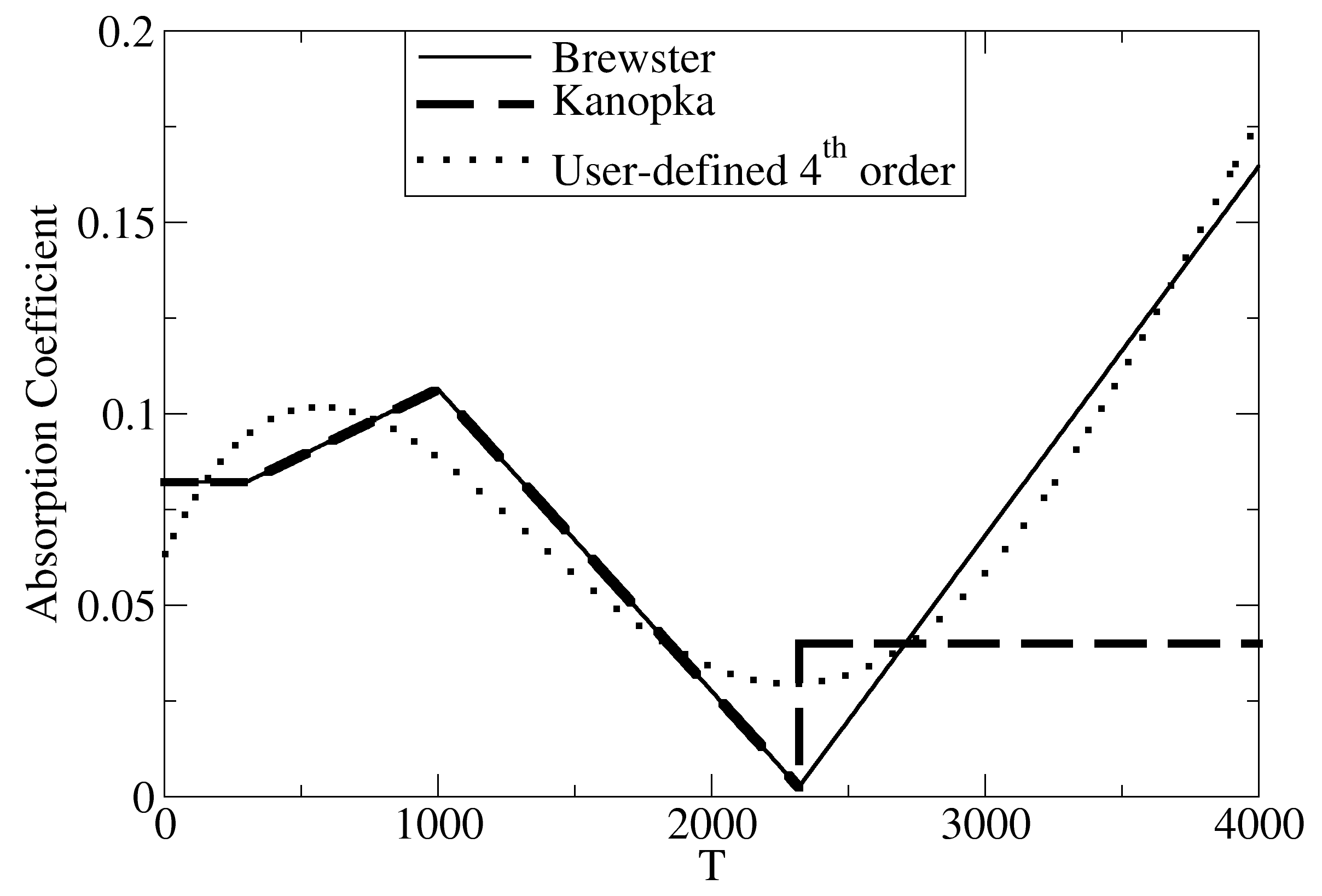
Fig. 3.23 Alumina absorption coefficient for standard models Brewster and Kanopka along with a user-specified model
3.3.7.4. Emission Multiplier
For propellant fire simulations which use the evaporating Lagrangian particle type, analysts have determined that modifying the particle-radiation coupling can be advantageous to reproducing experimental results. To address this, Fuego has a capability to modify the particle radiation emission with a constant multiplier. When the emission multiplier is not set, a default value of 1 is assumed, and emission equal to absorption when the particle and fluid temperatures are identical. Particle radiant emission  and absorption
  are:
are:
(3.736)
(3.737)
where  is the particle absorptivity,
  is the particle radius,
  is the Stefan-Boltzmann constant,
  are the particle and fluid temperatures respectively, and
  is the emission multiplier described above.
3.3.7.5. Lagrangian Particle Spray: Number Represented Function
Lagrangian particle sprays have historically been required to use parcelling (grouping of several particles into a single parcel) with either a constant mass represented per parcel or constant number represented per parcel. In propellant fire applications and other reacting particle environments, a more sophisticated functionality between the number of particles represented per parcel and particle size can increase the efficiency of simulations. For this reason, Fuego includes a capability to allow the analyst to specify this function (parcel size vs. particle diameter). This function is specified by a vector for each (number represented per parcel and diameter). For diameters at or below the lowest specified in the vector, the number represented is constant and equal to the value at the lowest diameter specified. For diameters at or above the highest specified in the vector, the number represented is constant and equal to the value at the largest diameter specified. Intermediate values are linearly interpolated. Figure 3.24 diagrams the way parcelling works for each of the different parcelling schemes.
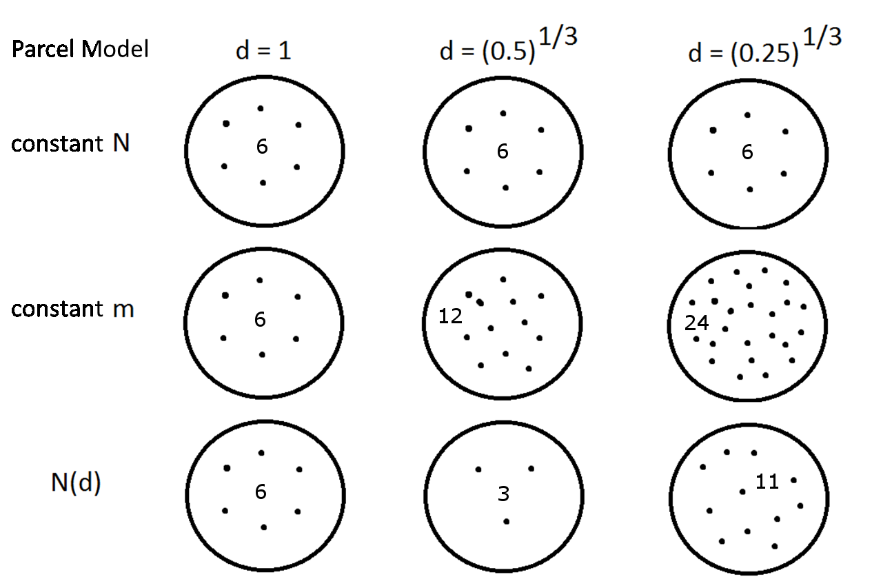
Fig. 3.24 For a Lagrangian particle spray, the number of particles contained within a parcel for three representative particle diameters using constant number, constant mass, and user defined number of particles per parcel. Circles represent parcels with the points inside representing the number of particles contained in the parcel.
3.3.7.6. Lagrangian Particle Insertion: User Definable Mechanism
Previous to version 4.30, Lagrangian particles could be inserted into the domain through two mechanisms: 1) batch introduction of a group of particles at a specified time with the particle configuration defined by a particle data file or a filled shape (i.e. cone, cylinder) with shape parameters or 2) via a particle spray with either a rectangular or circular nozzle and a specified mass flux rate. In cases where users needed a more novel insertion mechanism, Fuego lacked the capability. Fuego now includes a mechanism for particle insertion from file data in which users can specify not only particle positions, velocities, and diameters on insertion, but also particle temperature, number of particles per parcel, and insertion time. Through this method users have a full range of particle insertion options at their disposal. The dynamical form for particle introduction is contained within the file data, and does not rely on templated forms for static shapes or sprays, though those capabilities are still available. Users can, for instance, introduce particles from a very specific particle size distribution isotropically through the system with a rate of their choosing or create a particle spray with a conical nozzle with velocity vectors normal to the nozzle. The only limitation lies in the ability of the user to specify this mechanism through the particle data file. Figure 3.25 shows some examples of particle insertion types available with this capability. Figures Example of particle spread from a conical shaped particle spray nozzle at early times. This nonstandard spray form was generated through the particle creation from file data mechanism. Here particle temperatures are set to be a function of their position with the hottest particles leaving the nozzle near the circular base of the cone. and Same simulation as Figure %s but at late time display a conical particle spray generated with this mechanism from two different perspectives (conical axis lying in the plane of the figure and normal to the figure) at both early and late times in the simulation. In this case, the particle temperature has been designed to be a function of the position at which the particle left the spray nozzle. Many other forms are possible.
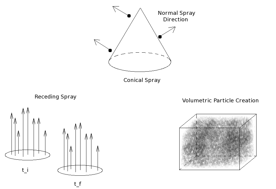
Fig. 3.25 Examples of particle insertion types that can be used with particle insert from file mechanism
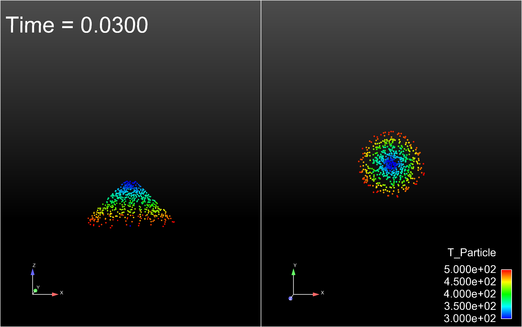
Fig. 3.26 Example of particle spread from a conical shaped particle spray nozzle at early times. This nonstandard spray form was generated through the particle creation from file data mechanism. Here particle temperatures are set to be a function of their position with the hottest particles leaving the nozzle near the circular base of the cone.
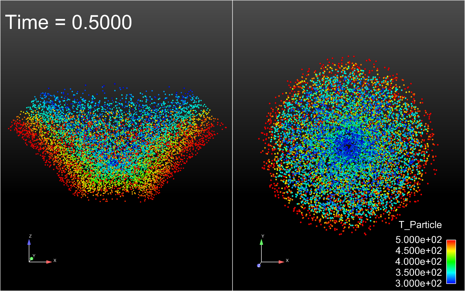
Fig. 3.27 Same simulation as Figure 3.26 but at late time