3.6. Radiation
3.6.1. Surface Radiation
A surface may exchange energy with its surroundings through thermal
radiation. Any incident surface radiation will be either transmitted,
reflected or absorbed. Letting  ,
,  and
and  represent
the fractions of the incident flux in each category then
represent
the fractions of the incident flux in each category then

and for no transmission

Using the Kirchhoff identity

then the reflectance is
(3.100)
where  is the emissivity.
In order to understand the radiative energy balance at a surface one considers the rate at which energy streams away from the surface, the radiosity, defined as
(3.101)
where  is the blackbody emissive power and
  is the irradiation.
Substituting for the reflectance (3.100) then
is the irradiation.
Substituting for the reflectance (3.100) then
(3.102)
The surface flux  is the difference between the energy that radiates away
and the incident energy
is the difference between the energy that radiates away
and the incident energy
(3.103)
and substitution for the radiosity we find that

When is derived from an external temperature interaction
this boundary condition is often called far-field radiation, since it usually
models the radiative transfer of energy between a surface and the
external environment. However, the boundary condition is found
to have more general utility when one considers its role in
modeling radiative transfer between two surfaces,  &
&  ,
as shown in Fig. 3.3, where
,
as shown in Fig. 3.3, where  is
analogous to
is
analogous to  .
.
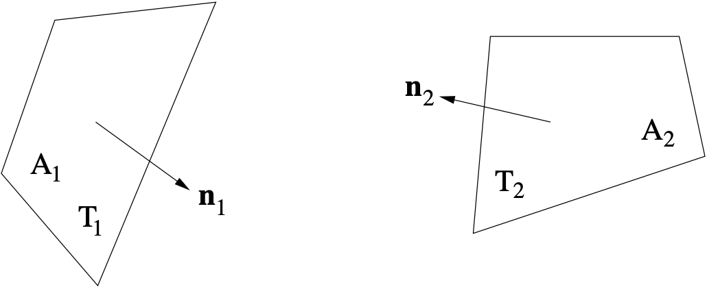
Fig. 3.3 Surface Radiative Exchange
For the case in which the temperature  is known and independent of temperature
  then
using the emissive power
then
using the emissive power  the normal flux per unit area across may be written as
(3.104)
where  denotes the Stefan-Boltzmann constant,
is the emissivity of the surface and
denotes the Stefan-Boltzmann constant,
is the emissivity of the surface and  is the form
factor. We remark that
(3.104) is a nonlinear boundary condition, since the
unknown temperature, is raised to the fourth power and furthermore the
emissivity may be a function of temperature. It is important
to note that the form factor may differ
from the more familiar view factor
is the form
factor. We remark that
(3.104) is a nonlinear boundary condition, since the
unknown temperature, is raised to the fourth power and furthermore the
emissivity may be a function of temperature. It is important
to note that the form factor may differ
from the more familiar view factor  encountered in
enclosure radiation problems. The question often asked is how does one
determine the appropriate value of form factor .
encountered in
enclosure radiation problems. The question often asked is how does one
determine the appropriate value of form factor .
The form factor can be best described using a
network analogy of radiative transfer between two surfaces as shown below.
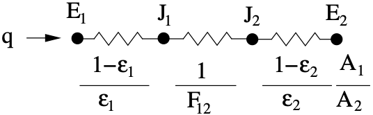
Fig. 3.4 Radiative Transfer Circuit Model
Using the emitted energy  and radiosity
  the network the heat flux can
be written in terms of a thermal resistance
the network the heat flux can
be written in terms of a thermal resistance  as
as
(3.105)
and from the network model

For  the third term of can be neglected and
  .
Comparing expressions (3.104) and (3.105) then
.
Comparing expressions (3.104) and (3.105) then

so estimation of is not required.
For  (black receiving surface) but
 and once again the third term of can
be neglected so that
and once again the third term of can
be neglected so that
(3.106)
If both surfaces are black  then
from the previous expression (3.106)
we find that
then
from the previous expression (3.106)
we find that  .
.
During a simulation the surface heat flux is integrated over the
spatial discretization of surface . Here we note that
defining the flux on a per unit area basis enables us to apply the
radiative flux (3.104) consistently with evaluated
for the entire surface even when the surface is discretized.
3.6.2. Enclosure Radiation
When energy radiates from one portion of a surface to another, and the intermediate medium is transparent (i.e., it does not absorb any energy), then enclosure radiation may be used to model the heat flux on the surface. Using the net radiation method [18], the normal flux at a particular location on the surface may be written as the difference between the emitted radiative heat flux leaving the surface, and the absorbed incident radiative flux due to the rest of the enclosure, namely
(3.107)
where denotes the absorptivity of the surface, and
represents the surface irradiation. Under the additional assumption
that the emissivity, absorptivity, and reflectivity are independent
of direction and wavelength, we may write
(3.108)
where is the reflectivity.
Without loss of generality, we can regard
the enclosure,  , as a
union of surfaces,
, as a
union of surfaces,

This situation is
illustrated in Fig. 3.6, where the radiosity for surface  in the enclosure is defined to be
(3.109)
where  is the area averaged constant temperature on facet
  computed via
(3.110)
The surface irradiation for surface is determined by the radiosity
of all the other surfaces in the enclosure through the relation
(3.111)
where  denotes the geometric viewfactor of surface with respect to
surface
denotes the geometric viewfactor of surface with respect to
surface  . The viewfactor may be considered as the fraction of energy that
leaves surface and arrives at surface . For a given pair of surfaces shown in Fig. 3.5,
the viewfactor is defined as the following integral
. The viewfactor may be considered as the fraction of energy that
leaves surface and arrives at surface . For a given pair of surfaces shown in Fig. 3.5,
the viewfactor is defined as the following integral
(3.112)
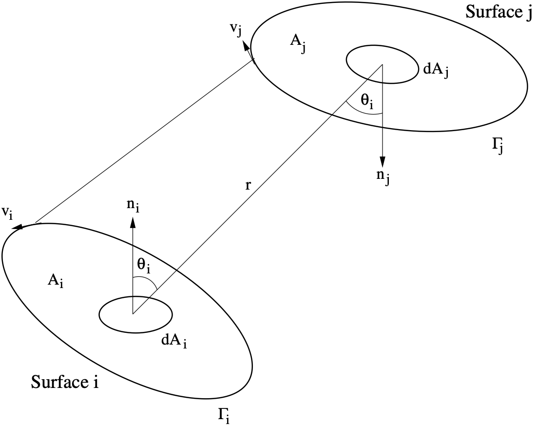
Fig. 3.5 Viewfactor Configuration.
Viewfactors are computed using the Chaparral library [19].
Determination of the viewfactors is a compute intensive endeavor. As such, extraneous calculations
are eliminated based upon the geometry. One example of this would be excluding this calculation for surfaces
which are not visible to each other. Moreover, from a geometric view of
enclosure surfaces, Fig. 3.5, one can conclude that
legitimate interactions between surfaces are those for which  and
and  are opposed. Thus an important feature of the enclosure model is the notion of
inward facing normals. This convention effectively defines the interaction
between the enclosure subfacets.
are opposed. Thus an important feature of the enclosure model is the notion of
inward facing normals. This convention effectively defines the interaction
between the enclosure subfacets.
Note
For closed surfaces (watertight enclosures), for each facet the
row-sum over all surface  facets should equal one, i.e.,
  .
.
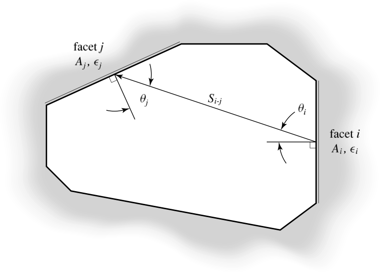
Fig. 3.6 Two arbitrary facets radiating energy to one another
in a radiation enclosure. The energy exchanged depends on:
the shape, orientation, distance, area  ,
,  ,
temperatures ,
,
temperatures ,  , and radiative properties of the
facets
, and radiative properties of the
facets  ,
,  .
.
Upon substitution of equations (3.111) and (3.108) into (3.109), the radiosity may be written as
(3.113)
Finally, the first  term in (3.113) may be moved inside the summation
to yield
term in (3.113) may be moved inside the summation
to yield
(3.114)![\sum\limits_{j = 1}^N {\left[ \delta_{ij} - (1 - \epsilon_i) F_{ij} \right] J_j}
= \sigma \epsilon_i \vartemp^4_i,](data:image/svg+xml;base64,PD94bWwgdmVyc2lvbj0nMS4wJyBlbmNvZGluZz0nVVRGLTgnPz4KPCEtLSBUaGlzIGZpbGUgd2FzIGdlbmVyYXRlZCBieSBkdmlzdmdtIDMuMC4zIC0tPgo8c3ZnIHZlcnNpb249JzEuMScgeG1sbnM9J2h0dHA6Ly93d3cudzMub3JnLzIwMDAvc3ZnJyB4bWxuczp4bGluaz0naHR0cDovL3d3dy53My5vcmcvMTk5OS94bGluaycgd2lkdGg9JzE5Mi43ODY3MjRwdCcgaGVpZ2h0PSc0Mi40Mzk4MjRwdCcgdmlld0JveD0nOTcuODc4MTIgLTQzLjgzNDU4NyAxOTIuNzg2NzI0IDQyLjQzOTgyNCc+CjxkZWZzPgo8cGF0aCBpZD0nZzEtMCcgZD0nTTkuMTkxNTMyLTMuMjA3OTdDOS40Mjg2NDMtMy4yMDc5NyA5LjY3OTcwMS0zLjIwNzk3IDkuNjc5NzAxLTMuNDg2OTI0UzkuNDI4NjQzLTMuNzY1ODc4IDkuMTkxNTMyLTMuNzY1ODc4SDEuNjQ1ODI4QzEuNDA4NzE3LTMuNzY1ODc4IDEuMTU3NjU5LTMuNzY1ODc4IDEuMTU3NjU5LTMuNDg2OTI0UzEuNDA4NzE3LTMuMjA3OTcgMS42NDU4MjgtMy4yMDc5N0g5LjE5MTUzMlonLz4KPHBhdGggaWQ9J2cwLTg4JyBkPSdNMTcuNjU3NzgzIDE5LjUyNjc3NUwxOS4zNDU0NTUgMTUuMDYzNTEySDE4Ljk5Njc2MkMxOC40NTI4MDIgMTYuNTE0MDcyIDE2Ljk3NDM0NiAxNy40NjI1MTYgMTUuMzcwMzYxIDE3Ljg4MDk0NkMxNS4wNzc0NiAxNy45NTA2ODUgMTMuNzEwNTg1IDE4LjMxMzMyNSAxMS4wMzI2MjggMTguMzEzMzI1SDIuNjIyMTY3TDkuNzIxNTQ0IDkuOTg2NTVDOS44MTkxNzggOS44NzQ5NjkgOS44NDcwNzMgOS44MzMxMjYgOS44NDcwNzMgOS43NjMzODdDOS44NDcwNzMgOS43MzU0OTIgOS44NDcwNzMgOS42OTM2NDkgOS43NDk0NCA5LjU1NDE3MkwzLjI0OTgxMyAuNjY5NDg5SDEwLjg5MzE1MUMxMi43NjIxNDIgLjY2OTQ4OSAxNC4wMzEzODIgLjg2NDc1NyAxNC4xNTY5MTIgLjg5MjY1M0MxNC45MTAwODcgMS4wMDQyMzQgMTYuMTIzNTM3IDEuMjQxMzQ1IDE3LjIyNTQwNSAxLjkzODczQzE3LjU3NDA5NyAyLjE2MTg5MyAxOC41MjI1NCAyLjc4OTUzOSAxOC45OTY3NjIgMy45MTkzMDNIMTkuMzQ1NDU1TDE3LjY1Nzc4MyAwSDEuMTcxNjA2Qy44NTA4MDkgMCAuODM2ODYyIC4wMTM5NDggLjc5NTAxOSAuMDk3NjM0Qy43ODEwNzEgLjEzOTQ3NyAuNzgxMDcxIC40MDQ0ODMgLjc4MTA3MSAuNTU3OTA4TDguMTU5NDAyIDEwLjY1NjA0TC45MzQ0OTYgMTkuMTIyMjkxQy43OTUwMTkgMTkuMjg5NjY0IC43OTUwMTkgMTkuMzU5NDAyIC43OTUwMTkgMTkuMzczMzVDLjc5NTAxOSAxOS41MjY3NzUgLjkyMDU0OCAxOS41MjY3NzUgMS4xNzE2MDYgMTkuNTI2Nzc1SDE3LjY1Nzc4M1onLz4KPHBhdGggaWQ9J2cyLTc4JyBkPSdNNy4zODEwODktNS42NDMyMTNDNy40Nzg3MjItNi4wMzM3NDcgNy42NTQ0NjItNi4zMzY0MTEgOC40MzU1My02LjM2NTcwMUM4LjQ4NDM0Ny02LjM2NTcwMSA4LjYwMTUwNy02LjM3NTQ2NCA4LjYwMTUwNy02LjU2MDk2OEM4LjYwMTUwNy02LjU3MDczMSA4LjYwMTUwNy02LjY2ODM2NCA4LjQ3NDU4My02LjY2ODM2NEM4LjE1MjM5My02LjY2ODM2NCA3LjgxMDY3Ni02LjYzOTA3NCA3LjQ4ODQ4NS02LjYzOTA3NEM3LjE1NjUzMi02LjYzOTA3NCA2LjgxNDgxNS02LjY2ODM2NCA2LjQ5MjYyNC02LjY2ODM2NEM2LjQzNDA0NC02LjY2ODM2NCA2LjMxNjg4NC02LjY2ODM2NCA2LjMxNjg4NC02LjQ3MzA5OEM2LjMxNjg4NC02LjM2NTcwMSA2LjQxNDUxNy02LjM2NTcwMSA2LjQ5MjYyNC02LjM2NTcwMUM3LjA0OTEzNS02LjM1NTkzNyA3LjE1NjUzMi02LjE1MDkwNyA3LjE1NjUzMi01LjkzNjExNEM3LjE1NjUzMi01LjkwNjgyNCA3LjEzNzAwNS01Ljc2MDM3MyA3LjEyNzI0Mi01LjczMTA4M0w2LjAzMzc0Ny0xLjM4NjM5NUwzLjg3NjA0OC02LjQ4Mjg2MUMzLjc5Nzk0MS02LjY1ODYwMSAzLjc4ODE3OC02LjY2ODM2NCAzLjU2MzYyMS02LjY2ODM2NEgyLjI1NTMzM0MyLjA2MDA2Ni02LjY2ODM2NCAxLjk3MjE5Ni02LjY2ODM2NCAxLjk3MjE5Ni02LjQ3MzA5OEMxLjk3MjE5Ni02LjM2NTcwMSAyLjA2MDA2Ni02LjM2NTcwMSAyLjI0NTU2OS02LjM2NTcwMUMyLjI5NDM4Ni02LjM2NTcwMSAyLjkwOTQ3Ny02LjM2NTcwMSAyLjkwOTQ3Ny02LjI3NzgzMUwxLjYwMTE4OS0xLjAzNDkxNUMxLjUwMzU1NS0uNjQ0MzgxIDEuMzM3NTc4LS4zMzE5NTQgLjU0Njc0Ny0uMzAyNjY0Qy40ODgxNjctLjMwMjY2NCAuMzgwNzctLjI5MjkgLjM4MDc3LS4xMDczOTdDLjM4MDc3LS4wMzkwNTMgLjQyOTU4NyAwIC41MDc2OTQgMEMuODIwMTIxIDAgMS4xNjE4MzgtLjAyOTI5IDEuNDg0MDI4LS4wMjkyOUMxLjgxNTk4Mi0uMDI5MjkgMi4xNjc0NjMgMCAyLjQ4OTY1MyAwQzIuNTM4NDcgMCAyLjY2NTM5MyAwIDIuNjY1MzkzLS4xOTUyNjdDMi42NjUzOTMtLjI5MjkgMi41Nzc1MjMtLjMwMjY2NCAyLjQ3MDEyNi0uMzAyNjY0QzEuOTAzODUyLS4zMjIxOSAxLjgyNTc0NS0uNTM2OTg0IDEuODI1NzQ1LS43MzIyNTFDMS44MjU3NDUtLjgwMDU5NCAxLjgzNTUwOS0uODQ5NDExIDEuODY0Nzk5LS45NTY4MDhMMy4xNTM1Ni02LjExMTg1NEMzLjE5MjYxNC02LjA1MzI3NCAzLjE5MjYxNC02LjAzMzc0NyAzLjI0MTQzLTUuOTM2MTE0TDUuNjcyNTAzLS4xODU1MDRDNS43NDA4NDctLjAxOTUyNyA1Ljc3MDEzNyAwIDUuODU4MDA3IDBDNS45NjU0MDQgMCA1Ljk2NTQwNC0uMDI5MjkgNi4wMTQyMi0uMjA1MDNMNy4zODEwODktNS42NDMyMTNaJy8+CjxwYXRoIGlkPSdnMi0xMDUnIGQ9J00yLjc3Mjc5LTYuMTAyMDlDMi43NzI3OS02LjI5NzM1NyAyLjYzNjEwMy02LjQ1MzU3MSAyLjQxMTU0Ni02LjQ1MzU3MUMyLjE0NzkzNi02LjQ1MzU3MSAxLjg4NDMyNi02LjE5OTcyNCAxLjg4NDMyNi01LjkzNjExNEMxLjg4NDMyNi01Ljc1MDYxIDIuMDIxMDEyLTUuNTg0NjMzIDIuMjU1MzMzLTUuNTg0NjMzQzIuNDc5ODktNS41ODQ2MzMgMi43NzI3OS01LjgwOTE5IDIuNzcyNzktNi4xMDIwOVpNMi4wMzA3NzYtMi40MzEwNzNDMi4xNDc5MzYtMi43MTQyMSAyLjE0NzkzNi0yLjczMzczNyAyLjI0NTU2OS0yLjk5NzM0N0MyLjMyMzY3Ni0zLjE5MjYxNCAyLjM3MjQ5My0zLjMyOTMwMSAyLjM3MjQ5My0zLjUxNDgwNEMyLjM3MjQ5My0zLjk1NDE1NSAyLjA2MDA2Ni00LjMxNTM5OCAxLjU3MTg5OS00LjMxNTM5OEMuNjU0MTQ0LTQuMzE1Mzk4IC4yODMxMzctMi44OTk3MTMgLjI4MzEzNy0yLjgxMTg0M0MuMjgzMTM3LTIuNzE0MjEgLjM4MDc3LTIuNzE0MjEgLjQwMDI5Ny0yLjcxNDIxQy40OTc5MzEtMi43MTQyMSAuNTA3Njk0LTIuNzMzNzM3IC41NTY1MTEtMi44ODk5NUMuODIwMTIxLTMuODA3NzA0IDEuMjEwNjU1LTQuMTAwNjA1IDEuNTQyNjA4LTQuMTAwNjA1QzEuNjIwNzE1LTQuMTAwNjA1IDEuNzg2NjkyLTQuMTAwNjA1IDEuNzg2NjkyLTMuNzg4MTc4QzEuNzg2NjkyLTMuNTgzMTQ4IDEuNzE4MzQ5LTMuMzc4MTE3IDEuNjc5Mjk1LTMuMjgwNDg0QzEuNjAxMTg5LTMuMDI2NjM3IDEuMTYxODM4LTEuODk0MDg5IDEuMDA1NjI1LTEuNDc0MjY1Qy45MDc5OTEtMS4yMjA0MTggLjc4MTA2OC0uODk4MjI4IC43ODEwNjgtLjY5MzE5N0MuNzgxMDY4LS4yMzQzMiAxLjExMzAyMSAuMTA3Mzk3IDEuNTgxNjYyIC4xMDczOTdDMi40OTk0MTYgLjEwNzM5NyAyLjg2MDY2LTEuMzA4Mjg4IDIuODYwNjYtMS4zOTYxNThDMi44NjA2Ni0xLjQ5Mzc5MiAyLjc3Mjc5LTEuNDkzNzkyIDIuNzQzNS0xLjQ5Mzc5MkMyLjY0NTg2Ni0xLjQ5Mzc5MiAyLjY0NTg2Ni0xLjQ2NDUwMiAyLjU5NzA1LTEuMzE4MDUyQzIuNDIxMzA5LS43MDI5NjEgMi4wOTkxMTktLjEwNzM5NyAxLjYwMTE4OS0uMTA3Mzk3QzEuNDM1MjEyLS4xMDczOTcgMS4zNjY4NjgtLjIwNTAzIDEuMzY2ODY4LS40Mjk1ODdDMS4zNjY4NjgtLjY3MzY3MSAxLjQyNTQ0OC0uODEwMzU4IDEuNjUwMDA1LTEuNDA1OTIyTDIuMDMwNzc2LTIuNDMxMDczWicvPgo8cGF0aCBpZD0nZzItMTA2JyBkPSdNMy44NzYwNDgtNi4xMDIwOUMzLjg3NjA0OC02LjI4NzU5NCAzLjczOTM2MS02LjQ1MzU3MSAzLjUwNTA0MS02LjQ1MzU3MUMzLjI4MDQ4NC02LjQ1MzU3MSAyLjk4NzU4My02LjIyOTAxNCAyLjk4NzU4My01LjkzNjExNEMyLjk4NzU4My01Ljc0MDg0NyAzLjEyNDI3LTUuNTg0NjMzIDMuMzQ4ODI3LTUuNTg0NjMzQzMuNjEyNDM4LTUuNTg0NjMzIDMuODc2MDQ4LTUuODM4NDggMy44NzYwNDgtNi4xMDIwOVpNMS45MTM2MTYgLjQ4ODE2N0MxLjcyODExMiAxLjIzMDE4MSAxLjI1OTQ3MSAxLjc4NjY5MiAuNzEyNzI0IDEuNzg2NjkyQy42NTQxNDQgMS43ODY2OTIgLjUwNzY5NCAxLjc4NjY5MiAuMzMxOTU0IDEuNjk4ODIyQy42MjQ4NTQgMS42MzA0NzkgLjc3MTMwNCAxLjM3NjYzMiAuNzcxMzA0IDEuMTgxMzY1Qy43NzEzMDQgMS4wMjUxNTEgLjY2MzkwNyAuODM5NjQ4IC40MDAyOTcgLjgzOTY0OEMuMTU2MjE0IC44Mzk2NDgtLjEyNjkyMyAxLjA0NDY3OC0uMTI2OTIzIDEuMzk2MTU4Qy0uMTI2OTIzIDEuNzg2NjkyIC4yNjM2MSAyLjAwMTQ4NiAuNzMyMjUxIDIuMDAxNDg2QzEuNDE1Njg1IDIuMDAxNDg2IDIuMzIzNjc2IDEuNDg0MDI4IDIuNTY3NzYgLjUxNzQ1N0wzLjQ2NTk4Ny0zLjA1NTkyN0MzLjUxNDgwNC0zLjI1MTE5NCAzLjUxNDgwNC0zLjM4Nzg4MSAzLjUxNDgwNC0zLjQxNzE3MUMzLjUxNDgwNC0zLjk3MzY4MSAzLjEwNDc0NC00LjMxNTM5OCAyLjYxNjU3Ni00LjMxNTM5OEMxLjYyMDcxNS00LjMxNTM5OCAxLjA2NDIwNS0yLjg5OTcxMyAxLjA2NDIwNS0yLjgxMTg0M0MxLjA2NDIwNS0yLjcxNDIxIDEuMTYxODM4LTIuNzE0MjEgMS4xODEzNjUtMi43MTQyMUMxLjI2OTIzNS0yLjcxNDIxIDEuMjc4OTk4LTIuNzIzOTczIDEuMzU3MTA1LTIuOTA5NDc3QzEuNjAxMTg5LTMuNTA1MDQxIDIuMDUwMzAyLTQuMTAwNjA1IDIuNTg3Mjg2LTQuMTAwNjA1QzIuNzIzOTczLTQuMTAwNjA1IDIuODk5NzEzLTQuMDYxNTUxIDIuODk5NzEzLTMuNjUxNDkxQzIuODk5NzEzLTMuNDI2OTM0IDIuODcwNDIzLTMuMzE5NTM3IDIuODMxMzctMy4xNTM1NkwxLjkxMzYxNiAuNDg4MTY3WicvPgo8cGF0aCBpZD0nZzQtNDknIGQ9J00yLjg3MDQyMy02LjI0ODU0MUMyLjg3MDQyMy02LjQ4Mjg2MSAyLjg3MDQyMy02LjUwMjM4OCAyLjY0NTg2Ni02LjUwMjM4OEMyLjA0MDUzOS01Ljg3NzUzNCAxLjE4MTM2NS01Ljg3NzUzNCAuODY4OTM4LTUuODc3NTM0Vi01LjU3NDg3QzEuMDY0MjA1LTUuNTc0ODcgMS42NDAyNDItNS41NzQ4NyAyLjE0NzkzNi01LjgyODcxN1YtLjc3MTMwNEMyLjE0NzkzNi0uNDE5ODI0IDIuMTE4NjQ2LS4zMDI2NjQgMS4yMzk5NDUtLjMwMjY2NEguOTI3NTE4VjBDMS4yNjkyMzUtLjAyOTI5IDIuMTE4NjQ2LS4wMjkyOSAyLjUwOTE4LS4wMjkyOVMzLjc0OTEyNC0uMDI5MjkgNC4wOTA4NDEgMFYtLjMwMjY2NEgzLjc3ODQxNEMyLjg5OTcxMy0uMzAyNjY0IDIuODcwNDIzLS40MTAwNiAyLjg3MDQyMy0uNzcxMzA0Vi02LjI0ODU0MVonLz4KPHBhdGggaWQ9J2c0LTUyJyBkPSdNMi44NzA0MjMtMS42MTA5NTJWLS43NjE1NDFDMi44NzA0MjMtLjQxMDA2IDIuODUwODk3LS4zMDI2NjQgMi4xMjg0MDktLjMwMjY2NEgxLjkyMzM3OVYwQzIuMzIzNjc2LS4wMjkyOSAyLjgzMTM3LS4wMjkyOSAzLjI0MTQzLS4wMjkyOVM0LjE2ODk0OC0uMDI5MjkgNC41NjkyNDUgMFYtLjMwMjY2NEg0LjM2NDIxNUMzLjY0MTcyOC0uMzAyNjY0IDMuNjIyMjAxLS40MTAwNiAzLjYyMjIwMS0uNzYxNTQxVi0xLjYxMDk1Mkg0LjU5ODUzNVYtMS45MTM2MTZIMy42MjIyMDFWLTYuMzU1OTM3QzMuNjIyMjAxLTYuNTUxMjA0IDMuNjIyMjAxLTYuNjA5Nzg0IDMuNDY1OTg3LTYuNjA5Nzg0QzMuMzc4MTE3LTYuNjA5Nzg0IDMuMzQ4ODI3LTYuNjA5Nzg0IDMuMjcwNzItNi40OTI2MjRMLjI3MzM3NC0xLjkxMzYxNlYtMS42MTA5NTJIMi44NzA0MjNaTTIuOTI5MDAzLTEuOTEzNjE2SC41NDY3NDdMMi45MjkwMDMtNS41NTUzNDNWLTEuOTEzNjE2WicvPgo8cGF0aCBpZD0nZzQtNjEnIGQ9J002LjcwNzQxOC0zLjE5MjYxNEM2Ljg1Mzg2OC0zLjE5MjYxNCA3LjAzOTM3Mi0zLjE5MjYxNCA3LjAzOTM3Mi0zLjM4Nzg4MVM2Ljg1Mzg2OC0zLjU4MzE0OCA2LjcxNzE4MS0zLjU4MzE0OEguODY4OTM4Qy43MzIyNTEtMy41ODMxNDggLjU0Njc0Ny0zLjU4MzE0OCAuNTQ2NzQ3LTMuMzg3ODgxUy43MzIyNTEtMy4xOTI2MTQgLjg3ODcwMS0zLjE5MjYxNEg2LjcwNzQxOFpNNi43MTcxODEtMS4yOTg1MjVDNi44NTM4NjgtMS4yOTg1MjUgNy4wMzkzNzItMS4yOTg1MjUgNy4wMzkzNzItMS40OTM3OTJTNi44NTM4NjgtMS42ODkwNTkgNi43MDc0MTgtMS42ODkwNTlILjg3ODcwMUMuNzMyMjUxLTEuNjg5MDU5IC41NDY3NDctMS42ODkwNTkgLjU0Njc0Ny0xLjQ5Mzc5MlMuNzMyMjUxLTEuMjk4NTI1IC44Njg5MzgtMS4yOTg1MjVINi43MTcxODFaJy8+CjxwYXRoIGlkPSdnNS00MCcgZD0nTTQuNTMzMDAxIDMuMzg5MjlDNC41MzMwMDEgMy4zNDc0NDcgNC41MzMwMDEgMy4zMTk1NTIgNC4yOTU4OSAzLjA4MjQ0MUMyLjkwMTEyMSAxLjY3MzcyNCAyLjEyMDA1LS42Mjc2NDYgMi4xMjAwNS0zLjQ3Mjk3NkMyLjEyMDA1LTYuMTc4ODI5IDIuNzc1NTkyLTguNTA4MDk1IDQuMzkzNTI0LTEwLjE1MzkyM0M0LjUzMzAwMS0xMC4yNzk0NTIgNC41MzMwMDEtMTAuMzA3MzQ3IDQuNTMzMDAxLTEwLjM0OTE5MUM0LjUzMzAwMS0xMC40MzI4NzcgNC40NjMyNjMtMTAuNDYwNzcyIDQuNDA3NDcyLTEwLjQ2MDc3MkM0LjIyNjE1Mi0xMC40NjA3NzIgMy4wODI0NDEtOS40NTY1MzggMi4zOTkwMDQtOC4wODk2NjRDMS42ODc2NzEtNi42ODA5NDYgMS4zNjY4NzQtNS4xODg1NDMgMS4zNjY4NzQtMy40NzI5NzZDMS4zNjY4NzQtMi4yMzE2MzEgMS41NjIxNDItLjU3MTg1NiAyLjI4NzQyMiAuOTIwNTQ4QzMuMTEwMzM2IDIuNTk0MjcxIDQuMjU0MDQ3IDMuNTAwODcyIDQuNDA3NDcyIDMuNTAwODcyQzQuNDYzMjYzIDMuNTAwODcyIDQuNTMzMDAxIDMuNDcyOTc2IDQuNTMzMDAxIDMuMzg5MjlaJy8+CjxwYXRoIGlkPSdnNS00MScgZD0nTTMuOTMzMjUtMy40NzI5NzZDMy45MzMyNS00LjUzMzAwMSAzLjc5Mzc3My02LjI2MjUxNiAzLjAxMjcwMi03Ljg4MDQ0OEMyLjE4OTc4OC05LjU1NDE3MiAxLjA0NjA3Ny0xMC40NjA3NzIgLjg5MjY1My0xMC40NjA3NzJDLjgzNjg2Mi0xMC40NjA3NzIgLjc2NzEyMy0xMC40MzI4NzcgLjc2NzEyMy0xMC4zNDkxOTFDLjc2NzEyMy0xMC4zMDczNDcgLjc2NzEyMy0xMC4yNzk0NTIgMS4wMDQyMzQtMTAuMDQyMzQxQzIuMzk5MDA0LTguNjMzNjI0IDMuMTgwMDc1LTYuMzMyMjU0IDMuMTgwMDc1LTMuNDg2OTI0QzMuMTgwMDc1LS43ODEwNzEgMi41MjQ1MzMgMS41NDgxOTQgLjkwNjYgMy4xOTQwMjJDLjc2NzEyMyAzLjMxOTU1MiAuNzY3MTIzIDMuMzQ3NDQ3IC43NjcxMjMgMy4zODkyOUMuNzY3MTIzIDMuNDcyOTc2IC44MzY4NjIgMy41MDA4NzIgLjg5MjY1MyAzLjUwMDg3MkMxLjA3Mzk3MyAzLjUwMDg3MiAyLjIxNzY4NCAyLjQ5NjYzOCAyLjkwMTEyMSAxLjEyOTc2M0MzLjYxMjQ1My0uMjkyOTAyIDMuOTMzMjUtMS43OTkyNTMgMy45MzMyNS0zLjQ3Mjk3NlonLz4KPHBhdGggaWQ9J2c1LTQ5JyBkPSdNNC4wMTY5MzYtOC45NDA0NzNDNC4wMTY5MzYtOS4yNjEyNyA0LjAxNjkzNi05LjI3NTIxOCAzLjczNzk4My05LjI3NTIxOEMzLjQwMzIzOC04Ljg5ODYzIDIuNzA1ODUzLTguMzgyNTY1IDEuMjY5MjQtOC4zODI1NjVWLTcuOTc4MDgyQzEuNTkwMDM3LTcuOTc4MDgyIDIuMjg3NDIyLTcuOTc4MDgyIDMuMDU0NTQ1LTguMzQwNzIyVi0xLjA3Mzk3M0MzLjA1NDU0NS0uNTcxODU2IDMuMDEyNzAyLS40MDQ0ODMgMS43ODUzMDUtLjQwNDQ4M0gxLjM1MjkyN1YwQzEuNzI5NTE0LS4wMjc4OTUgMy4wODI0NDEtLjAyNzg5NSAzLjU0MjcxNS0uMDI3ODk1UzUuMzQxOTY4LS4wMjc4OTUgNS43MTg1NTUgMFYtLjQwNDQ4M0g1LjI4NjE3N0M0LjA1ODc4LS40MDQ0ODMgNC4wMTY5MzYtLjU3MTg1NiA0LjAxNjkzNi0xLjA3Mzk3M1YtOC45NDA0NzNaJy8+CjxwYXRoIGlkPSdnNS02MScgZD0nTTkuNDE0Njk1LTQuNTE5MDU0QzkuNjA5OTYzLTQuNTE5MDU0IDkuODYxMDIxLTQuNTE5MDU0IDkuODYxMDIxLTQuNzcwMTEyQzkuODYxMDIxLTUuMDM1MTE4IDkuNjIzOTEtNS4wMzUxMTggOS40MTQ2OTUtNS4wMzUxMThIMS4xOTk1MDJDMS4wMDQyMzQtNS4wMzUxMTggLjc1MzE3Ni01LjAzNTExOCAuNzUzMTc2LTQuNzg0MDZDLjc1MzE3Ni00LjUxOTA1NCAuOTkwMjg2LTQuNTE5MDU0IDEuMTk5NTAyLTQuNTE5MDU0SDkuNDE0Njk1Wk05LjQxNDY5NS0xLjkyNDc4MkM5LjYwOTk2My0xLjkyNDc4MiA5Ljg2MTAyMS0xLjkyNDc4MiA5Ljg2MTAyMS0yLjE3NTg0MUM5Ljg2MTAyMS0yLjQ0MDg0NyA5LjYyMzkxLTIuNDQwODQ3IDkuNDE0Njk1LTIuNDQwODQ3SDEuMTk5NTAyQzEuMDA0MjM0LTIuNDQwODQ3IC43NTMxNzYtMi40NDA4NDcgLjc1MzE3Ni0yLjE4OTc4OEMuNzUzMTc2LTEuOTI0NzgyIC45OTAyODYtMS45MjQ3ODIgMS4xOTk1MDItMS45MjQ3ODJIOS40MTQ2OTVaJy8+CjxwYXRoIGlkPSdnNS05MScgZD0nTTMuNDg2OTI0IDMuNDg2OTI0VjIuOTcwODU5SDIuMTMzOTk4Vi05Ljk0NDcwN0gzLjQ4NjkyNFYtMTAuNDYwNzcySDEuNjE3OTMzVjMuNDg2OTI0SDMuNDg2OTI0WicvPgo8cGF0aCBpZD0nZzUtOTMnIGQ9J00yLjE2MTg5My0xMC40NjA3NzJILjI5MjkwMlYtOS45NDQ3MDdIMS42NDU4MjhWMi45NzA4NTlILjI5MjkwMlYzLjQ4NjkyNEgyLjE2MTg5M1YtMTAuNDYwNzcyWicvPgo8cGF0aCBpZD0nZzMtMTQnIGQ9J00zLjYyNjQwMS02LjA4MTE5NkMxLjg0MTA5Ni01LjY0ODgxNyAuNTU3OTA4LTMuNzkzNzczIC41NTc5MDgtMi4xNjE4OTNDLjU1NzkwOC0uNjY5NDg5IDEuNTYyMTQyIC4xNjczNzIgMi42Nzc5NTggLjE2NzM3MkM0LjMyMzc4NiAuMTY3MzcyIDUuNDM5NjAxLTIuMDkyMTU0IDUuNDM5NjAxLTMuOTQ3MTk4QzUuNDM5NjAxLTUuMjAyNDkxIDQuODUzNzk4LTUuOTY5NjE0IDQuNTA1MTA2LTYuNDI5ODg4QzMuOTg5MDQxLTcuMDg1NDMgMy4xNTIxNzktOC4xNTk0MDIgMy4xNTIxNzktOC44Mjg4OTJDMy4xNTIxNzktOS4wNjYwMDIgMy4zMzM0OTktOS40ODQ0MzMgMy45NDcxOTgtOS40ODQ0MzNDNC4zNzk1NzctOS40ODQ0MzMgNC42NDQ1ODMtOS4zMzEwMDkgNS4wNjMwMTQtOS4wOTM4OThDNS4xODg1NDMtOS4wMTAyMTIgNS41MDkzNC04LjgyODg5MiA1LjY5MDY2LTguODI4ODkyQzUuOTgzNTYyLTguODI4ODkyIDYuMTkyNzc3LTkuMTIxNzkzIDYuMTkyNzc3LTkuMzQ0OTU2QzYuMTkyNzc3LTkuNjA5OTYzIDUuOTgzNTYyLTkuNjUxODA2IDUuNDk1MzkyLTkuNzYzMzg3QzQuODM5ODUxLTkuOTAyODY0IDQuNjQ0NTgzLTkuOTAyODY0IDQuNDA3NDcyLTkuOTAyODY0UzIuODAzNDg3LTkuOTAyODY0IDIuODAzNDg3LTguNDgwMTk5QzIuODAzNDg3LTcuNzk2NzYyIDMuMTUyMTc5LTcuMDAxNzQzIDMuNjI2NDAxLTYuMDgxMTk2Wk0zLjc3OTgyNi01LjgxNjE4OUM0LjMwOTgzOC00LjcxNDMyMSA0LjUxOTA1NC00LjI5NTg5IDQuNTE5MDU0LTMuMzg5MjlDNC41MTkwNTQtMi4zMDEzNyAzLjkzMzI1LS4xMTE1ODIgMi42OTE5MDUtLjExMTU4MkMyLjE0Nzk0NS0uMTExNTgyIDEuMzY2ODc0LS40NzQyMjIgMS4zNjY4NzQtMS43NzEzNTdDMS4zNjY4NzQtMi42Nzc5NTggMS44ODI5MzktNS4zMTQwNzIgMy43Nzk4MjYtNS44MTYxODlaJy8+CjxwYXRoIGlkPSdnMy0xNScgZD0nTTQuMDU4NzgtMy4xNjYxMjdDNC4yNjc5OTUtMy4xNjYxMjcgNC41MDUxMDYtMy4xNjYxMjcgNC41MDUxMDYtMy4zODkyOUM0LjUwNTEwNi0zLjU3MDYxIDQuMzY1NjI5LTMuNTcwNjEgNC4xMTQ1Ny0zLjU3MDYxSDEuODU1MDQ0QzIuMjAzNzM2LTQuODM5ODUxIDMuMDI2NjUtNS42MDY5NzQgNC4yNjc5OTUtNS42MDY5NzRINC42NzI0NzhDNC45MDk1ODktNS42MDY5NzQgNS4xMTg4MDQtNS42MDY5NzQgNS4xMTg4MDQtNS44MzAxMzdDNS4xMTg4MDQtNi4wMTE0NTcgNC45NjUzOC02LjAxMTQ1NyA0LjcxNDMyMS02LjAxMTQ1N0g0LjI0MDFDMi41MjQ1MzMtNi4wMTE0NTcgLjY0MTU5NC00LjY0NDU4MyAuNjQxNTk0LTIuNDU0Nzk1Qy42NDE1OTQtLjkwNjYgMS42ODc2NzEgLjEzOTQ3NyAzLjA2ODQ5MyAuMTM5NDc3QzMuOTYxMTQ2IC4xMzk0NzcgNC44Mzk4NTEtLjQxODQzMSA0LjgzOTg1MS0uNTU3OTA4QzQuODM5ODUxLS42NDE1OTQgNC43OTgwMDctLjcyNTI4IDQuNzE0MzIxLS43MjUyOEM0LjY3MjQ3OC0uNzI1MjggNC42NDQ1ODMtLjcxMTMzMyA0LjU3NDg0NC0uNjU1NTQyQzQuMDQ0ODMyLS4zMDY4NDkgMy41Mjg3NjctLjEzOTQ3NyAzLjExMDMzNi0uMTM5NDc3QzIuMzcxMTA4LS4xMzk0NzcgMS41OTAwMzctLjYyNzY0NiAxLjU5MDAzNy0xLjk4MDU3M0MxLjU5MDAzNy0yLjI0NTU3OSAxLjYxNzkzMy0yLjYwODIxOSAxLjc0MzQ2Mi0zLjE2NjEyN0g0LjA1ODc4WicvPgo8cGF0aCBpZD0nZzMtMjcnIGQ9J003LjA4NTQzLTUuMjU4MjgxQzcuMjY2NzUtNS4yNTgyODEgNy43MjcwMjQtNS4yNTgyODEgNy43MjcwMjQtNS43MDQ2MDhDNy43MjcwMjQtNi4wMTE0NTcgNy40NjIwMTctNi4wMTE0NTcgNy4yMTA5NTktNi4wMTE0NTdINC4xMjg1MThDMi4wMzYzNjQtNi4wMTE0NTcgLjUzMDAxMi0zLjY4MjE5MiAuNTMwMDEyLTIuMDM2MzY0Qy41MzAwMTItLjg1MDgwOSAxLjI5NzEzNiAuMTM5NDc3IDIuNTUyNDI4IC4xMzk0NzdDNC4xOTgyNTcgLjEzOTQ3NyA1Ljk5NzUwOS0xLjYzMTg4IDUuOTk3NTA5LTMuNzI0MDM1QzUuOTk3NTA5LTQuMjY3OTk1IDUuODcxOTgtNC43OTgwMDcgNS41MzcyMzUtNS4yNTgyODFINy4wODU0M1pNMi41NjYzNzYtLjEzOTQ3N0MxLjg1NTA0NC0uMTM5NDc3IDEuMzM4OTc5LS42ODM0MzcgMS4zMzg5NzktMS42NDU4MjhDMS4zMzg5NzktMi40ODI2OSAxLjg0MTA5Ni01LjI1ODI4MSAzLjg5MTQwNy01LjI1ODI4MUM0LjQ5MTE1OC01LjI1ODI4MSA1LjE2MDY0OC00Ljk2NTM4IDUuMTYwNjQ4LTMuODkxNDA3QzUuMTYwNjQ4LTMuNDAzMjM4IDQuOTM3NDg0LTIuMjMxNjMxIDQuNDQ5MzE1LTEuNDIyNjY1QzMuOTQ3MTk4LS41OTk3NTEgMy4xOTQwMjItLjEzOTQ3NyAyLjU2NjM3Ni0uMTM5NDc3WicvPgo8cGF0aCBpZD0nZzMtNTknIGQ9J00yLjcxOTgwMSAuMDU1NzkxQzIuNzE5ODAxLS43NTMxNzYgMi40NTQ3OTUtMS4zNTI5MjcgMS44ODI5MzktMS4zNTI5MjdDMS40MzY2MTMtMS4zNTI5MjcgMS4yMTM0NS0uOTkwMjg2IDEuMjEzNDUtLjY4MzQzN1MxLjQyMjY2NSAwIDEuODk2ODg3IDBDMi4wNzgyMDcgMCAyLjIzMTYzMS0uMDU1NzkxIDIuMzU3MTYxLS4xODEzMkMyLjM4NTA1Ni0uMjA5MjE1IDIuMzk5MDA0LS4yMDkyMTUgMi40MTI5NTEtLjIwOTIxNUMyLjQ0MDg0Ny0uMjA5MjE1IDIuNDQwODQ3LS4wMTM5NDggMi40NDA4NDcgLjA1NTc5MUMyLjQ0MDg0NyAuNTE2MDY1IDIuMzU3MTYxIDEuNDIyNjY1IDEuNTQ4MTk0IDIuMzI5MjY1QzEuMzk0NzcgMi40OTY2MzggMS4zOTQ3NyAyLjUyNDUzMyAxLjM5NDc3IDIuNTUyNDI4QzEuMzk0NzcgMi42MjIxNjcgMS40NjQ1MDggMi42OTE5MDUgMS41MzQyNDcgMi42OTE5MDVDMS42NDU4MjggMi42OTE5MDUgMi43MTk4MDEgMS42NTk3NzYgMi43MTk4MDEgLjA1NTc5MVonLz4KPHBhdGggaWQ9J2czLTcwJyBkPSdNNC4xNDI0NjYtNC41NDY5NDlINS40ODE0NDVDNi41NDE0NjktNC41NDY5NDkgNi42MjUxNTYtNC4zMDk4MzggNi42MjUxNTYtMy45MDUzNTVDNi42MjUxNTYtMy43MjQwMzUgNi41OTcyNi0zLjUyODc2NyA2LjUyNzUyMi0zLjIyMTkxOEM2LjQ5OTYyNi0zLjE2NjEyNyA2LjQ4NTY3OS0zLjA5NjM4OSA2LjQ4NTY3OS0zLjA2ODQ5M0M2LjQ4NTY3OS0yLjk3MDg1OSA2LjU0MTQ2OS0yLjkxNTA2OCA2LjYzOTEwMy0yLjkxNTA2OEM2Ljc1MDY4NS0yLjkxNTA2OCA2Ljc2NDYzMy0yLjk3MDg1OSA2LjgyMDQyMy0zLjE5NDAyMkw3LjYyOTM5LTYuNDQzODM2QzcuNjI5MzktNi40OTk2MjYgNy41ODc1NDctNi41ODMzMTMgNy40ODk5MTMtNi41ODMzMTNDNy4zNjQzODQtNi41ODMzMTMgNy4zNTA0MzYtNi41Mjc1MjIgNy4yOTQ2NDUtNi4yOTA0MTFDNy4wMDE3NDMtNS4yNDQzMzQgNi43MjI3OS00Ljk1MTQzMiA1LjUwOTM0LTQuOTUxNDMySDQuMjQwMUw1LjE0NjctOC41NjM4ODVDNS4yNzIyMjktOS4wNTIwNTUgNS4zMDAxMjUtOS4wOTM4OTggNS44NzE5OC05LjA5Mzg5OEg3Ljc0MDk3MUM5LjQ4NDQzMy05LjA5Mzg5OCA5LjczNTQ5Mi04LjU3NzgzMyA5LjczNTQ5Mi03LjU4NzU0N0M5LjczNTQ5Mi03LjUwMzg2MSA5LjczNTQ5Mi03LjE5NzAxMSA5LjY5MzY0OS02LjgzNDM3MUM5LjY3OTcwMS02Ljc3ODU4IDkuNjUxODA2LTYuNTk3MjYgOS42NTE4MDYtNi41NDE0NjlDOS42NTE4MDYtNi40Mjk4ODggOS43MjE1NDQtNi4zODgwNDUgOS44MDUyMy02LjM4ODA0NUM5LjkwMjg2NC02LjM4ODA0NSA5Ljk1ODY1NS02LjQ0MzgzNiA5Ljk4NjU1LTYuNjk0ODk0TDEwLjI3OTQ1Mi05LjEzNTc0MUMxMC4yNzk0NTItOS4xNzc1ODQgMTAuMzA3MzQ3LTkuMzE3MDYxIDEwLjMwNzM0Ny05LjM0NDk1NkMxMC4zMDczNDctOS40OTgzODEgMTAuMTgxODE4LTkuNDk4MzgxIDkuOTMwNzYtOS40OTgzODFIMy4zMTk1NTJDMy4wNTQ1NDUtOS40OTgzODEgMi45MTUwNjgtOS40OTgzODEgMi45MTUwNjgtOS4yNDczMjNDMi45MTUwNjgtOS4wOTM4OTggMy4wMTI3MDItOS4wOTM4OTggMy4yNDk4MTMtOS4wOTM4OThDNC4xMTQ1Ny05LjA5Mzg5OCA0LjExNDU3LTguOTk2MjY0IDQuMTE0NTctOC44NDI4MzlDNC4xMTQ1Ny04Ljc3MzEwMSA0LjEwMDYyMy04LjcxNzMxIDQuMDU4NzgtOC41NjM4ODVMMi4xNzU4NDEtMS4wMzIxM0MyLjA1MDMxMS0uNTQzOTYgMi4wMjI0MTYtLjQwNDQ4MyAxLjA0NjA3Ny0uNDA0NDgzQy43ODEwNzEtLjQwNDQ4MyAuNjQxNTk0LS40MDQ0ODMgLjY0MTU5NC0uMTUzNDI1Qy42NDE1OTQgMCAuNzY3MTIzIDAgLjg1MDgwOSAwQzEuMTE1ODE2IDAgMS4zOTQ3Ny0uMDI3ODk1IDEuNjU5Nzc2LS4wMjc4OTVIMy40NzI5NzZDMy43Nzk4MjYtLjAyNzg5NSA0LjExNDU3IDAgNC40MjE0MiAwQzQuNTQ2OTQ5IDAgNC43MTQzMjEgMCA0LjcxNDMyMS0uMjUxMDU5QzQuNzE0MzIxLS40MDQ0ODMgNC42MzA2MzUtLjQwNDQ4MyA0LjMyMzc4Ni0uNDA0NDgzQzMuMjIxOTE4LS40MDQ0ODMgMy4xOTQwMjItLjUwMjExNyAzLjE5NDAyMi0uNzExMzMzQzMuMTk0MDIyLS43ODEwNzEgMy4yMjE5MTgtLjg5MjY1MyAzLjI0OTgxMy0uOTkwMjg2TDQuMTQyNDY2LTQuNTQ2OTQ5WicvPgo8cGF0aCBpZD0nZzMtNzQnIGQ9J003LjQ0ODA3LTguNTYzODg1QzcuNTU5NjUxLTguOTgyMzE2IDcuNTg3NTQ3LTkuMTIxNzkzIDguMjcwOTg0LTkuMTIxNzkzQzguNDk0MTQ3LTkuMTIxNzkzIDguNjMzNjI0LTkuMTIxNzkzIDguNjMzNjI0LTkuMzcyODUyQzguNjMzNjI0LTkuNTI2Mjc2IDguNTA4MDk1LTkuNTI2Mjc2IDguNDUyMzA0LTkuNTI2Mjc2QzguMjE1MTkzLTkuNTI2Mjc2IDcuOTUwMTg3LTkuNDk4MzgxIDcuNjk5MTI4LTkuNDk4MzgxSDYuOTMyMDA1QzYuMzQ2MjAyLTkuNDk4MzgxIDUuNzMyNTAzLTkuNTI2Mjc2IDUuMTQ2Ny05LjUyNjI3NkM1LjAyMTE3MS05LjUyNjI3NiA0Ljg1Mzc5OC05LjUyNjI3NiA0Ljg1Mzc5OC05LjI3NTIxOEM0Ljg1Mzc5OC05LjEzNTc0MSA0Ljk2NTM4LTkuMTM1NzQxIDQuOTY1MzgtOS4xMjE3OTNINS4zMTQwNzJDNi40Mjk4ODgtOS4xMjE3OTMgNi40Mjk4ODgtOS4wMTAyMTIgNi40Mjk4ODgtOC44MDA5OTZDNi40Mjk4ODgtOC43ODcwNDkgNi40Mjk4ODgtOC42ODk0MTUgNi4zNzQwOTctOC40NjYyNTJMNC43NzAxMTItMi4wOTIxNTRDNC40MDc0NzItLjY2OTQ4OSAzLjQ3Mjk3NiAuMDEzOTQ4IDIuODAzNDg3IC4wMTM5NDhDMi4zMjkyNjUgLjAxMzk0OCAxLjY1OTc3Ni0uMjA5MjE1IDEuNDkyNDAzLS45NDg0NDNDMS41NDgxOTQtLjkzNDQ5NiAxLjYxNzkzMy0uOTIwNTQ4IDEuNjczNzI0LS45MjA1NDhDMi4xMzM5OTgtLjkyMDU0OCAyLjQ5NjYzOC0xLjMyNTAzMSAyLjQ5NjYzOC0xLjcyOTUxNEMyLjQ5NjYzOC0xLjk1MjY3NyAyLjM1NzE2MS0yLjI0NTU3OSAxLjkzODczLTIuMjQ1NTc5QzEuNjg3NjcxLTIuMjQ1NTc5IDEuMTAxODY4LTIuMTA2MTAyIDEuMTAxODY4LTEuMTk5NTAyQzEuMTAxODY4LS4zMjA3OTcgMS44MjcxNDggLjI5MjkwMiAyLjgzMTM4MiAuMjkyOTAyQzQuMTAwNjIzIC4yOTI5MDIgNS40Njc0OTctLjY2OTQ4OSA1LjgwMjI0Mi0xLjk5NDUyMUw3LjQ0ODA3LTguNTYzODg1WicvPgo8cGF0aCBpZD0nZzMtODQnIGQ9J001LjgxNjE4OS04LjUwODA5NUM1Ljg5OTg3NS04Ljg0MjgzOSA1LjkyNzc3MS04Ljk2ODM2OSA2LjEzNjk4Ni05LjAyNDE1OUM2LjI0ODU2OC05LjA1MjA1NSA2LjcwODg0Mi05LjA1MjA1NSA3LjAwMTc0My05LjA1MjA1NUM4LjM5NjUxMy05LjA1MjA1NSA5LjA1MjA1NS04Ljk5NjI2NCA5LjA1MjA1NS03LjkwODM0NEM5LjA1MjA1NS03LjY5OTEyOCA4Ljk5NjI2NC03LjE2OTExNiA4LjkxMjU3OC02LjY1MzA1MUw4Ljg5ODYzLTYuNDg1Njc5QzguODk4NjMtNi40Mjk4ODggOC45NTQ0MjEtNi4zNDYyMDIgOS4wMzgxMDctNi4zNDYyMDJDOS4xNzc1ODQtNi4zNDYyMDIgOS4xNzc1ODQtNi40MTU5NCA5LjIxOTQyNy02LjYzOTEwM0w5LjYyMzkxLTkuMTA3ODQ2QzkuNjUxODA2LTkuMjMzMzc1IDkuNjUxODA2LTkuMjYxMjcgOS42NTE4MDYtOS4zMDMxMTNDOS42NTE4MDYtOS40NTY1MzggOS41NjgxMi05LjQ1NjUzOCA5LjI4OTE2Ni05LjQ1NjUzOEgxLjY1OTc3NkMxLjMzODk3OS05LjQ1NjUzOCAxLjMyNTAzMS05LjQ0MjU5IDEuMjQxMzQ1LTkuMTkxNTMyTC4zOTA1MzUtNi42ODA5NDZDLjM3NjU4OC02LjY1MzA1MSAuMzM0NzQ1LTYuNDk5NjI2IC4zMzQ3NDUtNi40ODU2NzlDLjMzNDc0NS02LjQxNTk0IC4zOTA1MzUtNi4zNDYyMDIgLjQ3NDIyMi02LjM0NjIwMkMuNTg1ODAzLTYuMzQ2MjAyIC42MTM2OTktNi40MDE5OTMgLjY2OTQ4OS02LjU4MzMxM0MxLjI1NTI5My04LjI3MDk4NCAxLjU0ODE5NC05LjA1MjA1NSAzLjQwMzIzOC05LjA1MjA1NUg0LjMzNzczM0M0LjY3MjQ3OC05LjA1MjA1NSA0LjgxMTk1NS05LjA1MjA1NSA0LjgxMTk1NS04Ljg5ODYzQzQuODExOTU1LTguODU2Nzg3IDQuODExOTU1LTguODI4ODkyIDQuNzQyMjE3LTguNTc3ODMzTDIuODczMjI1LTEuMDg3OTJDMi43MzM3NDgtLjU0Mzk2IDIuNzA1ODUzLS40MDQ0ODMgMS4yMjczOTctLjQwNDQ4M0MuODc4NzA1LS40MDQ0ODMgLjc4MTA3MS0uNDA0NDgzIC43ODEwNzEtLjEzOTQ3N0MuNzgxMDcxIDAgLjkzNDQ5NiAwIDEuMDA0MjM0IDBDMS4zNTI5MjcgMCAxLjcxNTU2Ny0uMDI3ODk1IDIuMDY0MjU5LS4wMjc4OTVINC4yNDAxQzQuNTg4NzkyLS4wMjc4OTUgNC45NjUzOCAwIDUuMzE0MDcyIDBDNS40Njc0OTcgMCA1LjYwNjk3NCAwIDUuNjA2OTc0LS4yNjUwMDZDNS42MDY5NzQtLjQwNDQ4MyA1LjUwOTM0LS40MDQ0ODMgNS4xNDY3LS40MDQ0ODNDMy44OTE0MDctLjQwNDQ4MyAzLjg5MTQwNy0uNTMwMDEyIDMuODkxNDA3LS43MzkyMjhDMy44OTE0MDctLjc1MzE3NiAzLjg5MTQwNy0uODUwODA5IDMuOTQ3MTk4LTEuMDczOTczTDUuODE2MTg5LTguNTA4MDk1WicvPgo8L2RlZnM+CjxnIGlkPSdwYWdlMSc+Cjx1c2UgeD0nMTAzLjQ5Njk3MicgeT0nLTM3LjE2Mjk3NicgeGxpbms6aHJlZj0nI2cyLTc4Jy8+Cjx1c2UgeD0nOTcuODc4MTInIHk9Jy0zMi45Nzg2NzEnIHhsaW5rOmhyZWY9JyNnMC04OCcvPgo8dXNlIHg9Jzk5LjQyNDAzNScgeT0nLTMuMjkzMTkzJyB4bGluazpocmVmPScjZzItMTA2Jy8+Cjx1c2UgeD0nMTA0LjAwMzUyNycgeT0nLTMuMjkzMTkzJyB4bGluazpocmVmPScjZzQtNjEnLz4KPHVzZSB4PScxMTEuNTk3MjY3JyB5PSctMy4yOTMxOTMnIHhsaW5rOmhyZWY9JyNnNC00OScvPgo8dXNlIHg9JzEyMC4zNDk0NCcgeT0nLTE5LjcyODI4JyB4bGluazpocmVmPScjZzUtOTEnLz4KPHVzZSB4PScxMjQuMTQzMDQ1JyB5PSctMTkuNzI4MjgnIHhsaW5rOmhyZWY9JyNnMy0xNCcvPgo8dXNlIHg9JzEzMC4xOTE4MScgeT0nLTE3LjYzNjEzNScgeGxpbms6aHJlZj0nI2cyLTEwNScvPgo8dXNlIHg9JzEzMy41NTU0MDgnIHk9Jy0xNy42MzYxMzUnIHhsaW5rOmhyZWY9JyNnMi0xMDYnLz4KPHVzZSB4PScxNDEuNzMyNDg2JyB5PSctMTkuNzI4MjgnIHhsaW5rOmhyZWY9JyNnMS0wJy8+Cjx1c2UgeD0nMTU1LjY4MDE5MycgeT0nLTE5LjcyODI4JyB4bGluazpocmVmPScjZzUtNDAnLz4KPHVzZSB4PScxNjAuOTkxMjQnIHk9Jy0xOS43MjgyOCcgeGxpbms6aHJlZj0nI2c1LTQ5Jy8+Cjx1c2UgeD0nMTcwLjkxOTE5JyB5PSctMTkuNzI4MjgnIHhsaW5rOmhyZWY9JyNnMS0wJy8+Cjx1c2UgeD0nMTg0Ljg2Njg5NycgeT0nLTE5LjcyODI4JyB4bGluazpocmVmPScjZzMtMTUnLz4KPHVzZSB4PScxOTAuMzgxMzUyJyB5PSctMTcuNjM2MTM1JyB4bGluazpocmVmPScjZzItMTA1Jy8+Cjx1c2UgeD0nMTk0LjI0MzA3NicgeT0nLTE5LjcyODI4JyB4bGluazpocmVmPScjZzUtNDEnLz4KPHVzZSB4PScxOTkuNTU0MTIyJyB5PSctMTkuNzI4MjgnIHhsaW5rOmhyZWY9JyNnMy03MCcvPgo8dXNlIHg9JzIwOC4zOTQ4NzEnIHk9Jy0xNy42MzYxMzUnIHhsaW5rOmhyZWY9JyNnMi0xMDUnLz4KPHVzZSB4PScyMTEuNzU4NDY5JyB5PSctMTcuNjM2MTM1JyB4bGluazpocmVmPScjZzItMTA2Jy8+Cjx1c2UgeD0nMjE2LjgzNjA4NicgeT0nLTE5LjcyODI4JyB4bGluazpocmVmPScjZzUtOTMnLz4KPHVzZSB4PScyMjIuOTU0MjUxJyB5PSctMTkuNzI4MjgnIHhsaW5rOmhyZWY9JyNnMy03NCcvPgo8dXNlIHg9JzIzMC41MDI3NjYnIHk9Jy0xNy42MzYxMzUnIHhsaW5rOmhyZWY9JyNnMi0xMDYnLz4KPHVzZSB4PScyMzkuNDU0NzA2JyB5PSctMTkuNzI4MjgnIHhsaW5rOmhyZWY9JyNnNS02MScvPgo8dXNlIHg9JzI1My45NTExMjYnIHk9Jy0xOS43MjgyOCcgeGxpbms6aHJlZj0nI2czLTI3Jy8+Cjx1c2UgeD0nMjYyLjIxMzkzMycgeT0nLTE5LjcyODI4JyB4bGluazpocmVmPScjZzMtMTUnLz4KPHVzZSB4PScyNjcuNzI4Mzg3JyB5PSctMTcuNjM2MTM1JyB4bGluazpocmVmPScjZzItMTA1Jy8+Cjx1c2UgeD0nMjcxLjU5MDExMScgeT0nLTE5LjcyODI4JyB4bGluazpocmVmPScjZzMtODQnLz4KPHVzZSB4PScyODEuNDkxNDInIHk9Jy0yNS40ODcxNzInIHhsaW5rOmhyZWY9JyNnNC01MicvPgo8dXNlIHg9JzI3OS41OTQ2MTcnIHk9Jy0xNi4yODAxODInIHhsaW5rOmhyZWY9JyNnMi0xMDUnLz4KPHVzZSB4PScyODYuODcxMjM5JyB5PSctMTkuNzI4MjgnIHhsaW5rOmhyZWY9JyNnMy01OScvPgo8L2c+Cjwvc3ZnPgo8IS0tIERFUFRIPTAgLS0+)
where

(3.114) is a system of equations that can be solved for the unknown radiosity at each face.
Finally, we may rewrite (3.107) to express the radiative heat flux on
surface as
(3.115)
where  is given by (3.111) and depends on the unknown radiosity.
This heat flux is applied as a boundary condition to the appropriate energy equations, thereby fully coupling
the enclosure radiation problem with the volume energy equations.
is given by (3.111) and depends on the unknown radiosity.
This heat flux is applied as a boundary condition to the appropriate energy equations, thereby fully coupling
the enclosure radiation problem with the volume energy equations.
Instead of solving the monolithic equation system by forming the jacobian for the combined coupled system of equation systems, a segregated approach is used. At each nonlinear iteration, the radiosity equation is solved separately with the right hand side computed from the average facet temperature (3.110) using the current nonlinear temperature solution. Subsequently, the irradiation is computed from the radiosity in order to compute the heat flux contribution given by (3.115). A Newton step is then performed where the jacobian contribution of the radiative flux is computed as
(3.116)
where  is the
  nonlinear temperature residual,
  the test function and where
(3.117)
Here, the facet temperature given by (3.110) has been relabeled to  to avoid confusion with the nodal finite element temperature solution. The sensitivity of the radiative
heat flux with respect to the facet temperature is approximated as
to avoid confusion with the nodal finite element temperature solution. The sensitivity of the radiative
heat flux with respect to the facet temperature is approximated as
(3.118)![\dfrac{\partial q_n}{\partial T^e} = 4 \sigma \epsilon^e \left[T^e\right]^3](data:image/svg+xml;base64,PD94bWwgdmVyc2lvbj0nMS4wJyBlbmNvZGluZz0nVVRGLTgnPz4KPCEtLSBUaGlzIGZpbGUgd2FzIGdlbmVyYXRlZCBieSBkdmlzdmdtIDMuMC4zIC0tPgo8c3ZnIHZlcnNpb249JzEuMScgeG1sbnM9J2h0dHA6Ly93d3cudzMub3JnLzIwMDAvc3ZnJyB4bWxuczp4bGluaz0naHR0cDovL3d3dy53My5vcmcvMTk5OS94bGluaycgd2lkdGg9Jzk3Ljg2ODg1OHB0JyBoZWlnaHQ9JzI4LjY4OTAzcHQnIHZpZXdCb3g9JzE0NS42ODU3NDkgLTI4LjY4OTA0NSA5Ny44Njg4NTggMjguNjg5MDMnPgo8ZGVmcz4KPHBhdGggaWQ9J2cyLTUxJyBkPSdNMi44MzEzNy0zLjQzNjY5N0MzLjYzMTk2NC0zLjcwMDMwOCA0LjE5ODIzOC00LjM4Mzc0MiA0LjE5ODIzOC01LjE1NTA0NkM0LjE5ODIzOC01Ljk1NTY0IDMuMzM5MDY0LTYuNTAyMzg4IDIuNDAxNzgzLTYuNTAyMzg4QzEuNDE1Njg1LTYuNTAyMzg4IC42NzM2NzEtNS45MTY1ODcgLjY3MzY3MS01LjE3NDU3M0MuNjczNjcxLTQuODUyMzgyIC44ODg0NjQtNC42NjY4NzkgMS4xNzE2MDEtNC42NjY4NzlDMS40NzQyNjUtNC42NjY4NzkgMS42Njk1MzItNC44ODE2NzIgMS42Njk1MzItNS4xNjQ4MDlDMS42Njk1MzItNS42NTI5NzcgMS4yMTA2NTUtNS42NTI5NzcgMS4wNjQyMDUtNS42NTI5NzdDMS4zNjY4NjgtNi4xMzEzOCAyLjAxMTI0OS02LjI1ODMwNCAyLjM2MjcyOS02LjI1ODMwNEMyLjc2MzAyNy02LjI1ODMwNCAzLjMwMDAxMS02LjA0MzUxIDMuMzAwMDExLTUuMTY0ODA5QzMuMzAwMDExLTUuMDQ3NjQ5IDMuMjgwNDg0LTQuNDgxMzc1IDMuMDI2NjM3LTQuMDUxNzg4QzIuNzMzNzM3LTMuNTgzMTQ4IDIuNDAxNzgzLTMuNTUzODU3IDIuMTU3Njk5LTMuNTQ0MDk0QzIuMDc5NTkyLTMuNTM0MzMxIDEuODQ1MjcyLTMuNTE0ODA0IDEuNzc2OTI5LTMuNTE0ODA0QzEuNjk4ODIyLTMuNTA1MDQxIDEuNjMwNDc5LTMuNDk1Mjc3IDEuNjMwNDc5LTMuMzk3NjQ0QzEuNjMwNDc5LTMuMjkwMjQ3IDEuNjk4ODIyLTMuMjkwMjQ3IDEuODY0Nzk5LTMuMjkwMjQ3SDIuMjk0Mzg2QzMuMDk0OTgtMy4yOTAyNDcgMy40NTYyMjQtMi42MjYzNCAzLjQ1NjIyNC0xLjY2OTUzMkMzLjQ1NjIyNC0uMzQxNzE3IDIuNzgyNTUzLS4wNTg1OCAyLjM1Mjk2Ni0uMDU4NThDMS45MzMxNDItLjA1ODU4IDEuMjAwODkxLS4yMjQ1NTcgLjg1OTE3NC0uODAwNTk0QzEuMjAwODkxLS43NTE3NzggMS41MDM1NTUtLjk2NjU3MSAxLjUwMzU1NS0xLjMzNzU3OEMxLjUwMzU1NS0xLjY4OTA1OSAxLjIzOTk0NS0xLjg4NDMyNiAuOTU2ODA4LTEuODg0MzI2Qy43MjI0ODgtMS44ODQzMjYgLjQxMDA2LTEuNzQ3NjM5IC40MTAwNi0xLjMxODA1MkMuNDEwMDYtLjQyOTU4NyAxLjMxODA1MiAuMjE0Nzk0IDIuMzgyMjU2IC4yMTQ3OTRDMy41NzMzODQgLjIxNDc5NCA0LjQ2MTg0OS0uNjczNjcxIDQuNDYxODQ5LTEuNjY5NTMyQzQuNDYxODQ5LTIuNDcwMTI2IDMuODQ2NzU4LTMuMjMxNjY3IDIuODMxMzctMy40MzY2OTdaJy8+CjxwYXRoIGlkPSdnMy01MicgZD0nTTUuMDM1MTE4LTkuMDc5OTVDNS4wMzUxMTgtOS4zNDQ5NTYgNS4wMzUxMTgtOS40MTQ2OTUgNC44Mzk4NTEtOS40MTQ2OTVDNC43MjgyNjktOS40MTQ2OTUgNC42ODY0MjYtOS40MTQ2OTUgNC41NzQ4NDQtOS4yNDczMjNMLjM3NjU4OC0yLjczMzc0OFYtMi4zMjkyNjVINC4wNDQ4MzJWLTEuMDYwMDI1QzQuMDQ0ODMyLS41NDM5NiA0LjAxNjkzNi0uNDA0NDgzIDIuOTk4NzU1LS40MDQ0ODNIMi43MTk4MDFWMEMzLjA0MDU5OC0uMDI3ODk1IDQuMTQyNDY2LS4wMjc4OTUgNC41MzMwMDEtLjAyNzg5NVM2LjAzOTM1Mi0uMDI3ODk1IDYuMzYwMTQ5IDBWLS40MDQ0ODNINi4wODExOTZDNS4wNzY5NjEtLjQwNDQ4MyA1LjAzNTExOC0uNTQzOTYgNS4wMzUxMTgtMS4wNjAwMjVWLTIuMzI5MjY1SDYuNDQzODM2Vi0yLjczMzc0OEg1LjAzNTExOFYtOS4wNzk5NVpNNC4xMTQ1Ny03Ljk5MjAzVi0yLjczMzc0OEguNzI1MjhMNC4xMTQ1Ny03Ljk5MjAzWicvPgo8cGF0aCBpZD0nZzMtNjEnIGQ9J005LjQxNDY5NS00LjUxOTA1NEM5LjYwOTk2My00LjUxOTA1NCA5Ljg2MTAyMS00LjUxOTA1NCA5Ljg2MTAyMS00Ljc3MDExMkM5Ljg2MTAyMS01LjAzNTExOCA5LjYyMzkxLTUuMDM1MTE4IDkuNDE0Njk1LTUuMDM1MTE4SDEuMTk5NTAyQzEuMDA0MjM0LTUuMDM1MTE4IC43NTMxNzYtNS4wMzUxMTggLjc1MzE3Ni00Ljc4NDA2Qy43NTMxNzYtNC41MTkwNTQgLjk5MDI4Ni00LjUxOTA1NCAxLjE5OTUwMi00LjUxOTA1NEg5LjQxNDY5NVpNOS40MTQ2OTUtMS45MjQ3ODJDOS42MDk5NjMtMS45MjQ3ODIgOS44NjEwMjEtMS45MjQ3ODIgOS44NjEwMjEtMi4xNzU4NDFDOS44NjEwMjEtMi40NDA4NDcgOS42MjM5MS0yLjQ0MDg0NyA5LjQxNDY5NS0yLjQ0MDg0N0gxLjE5OTUwMkMxLjAwNDIzNC0yLjQ0MDg0NyAuNzUzMTc2LTIuNDQwODQ3IC43NTMxNzYtMi4xODk3ODhDLjc1MzE3Ni0xLjkyNDc4MiAuOTkwMjg2LTEuOTI0NzgyIDEuMTk5NTAyLTEuOTI0NzgySDkuNDE0Njk1WicvPgo8cGF0aCBpZD0nZzMtOTEnIGQ9J00zLjQ4NjkyNCAzLjQ4NjkyNFYyLjk3MDg1OUgyLjEzMzk5OFYtOS45NDQ3MDdIMy40ODY5MjRWLTEwLjQ2MDc3MkgxLjYxNzkzM1YzLjQ4NjkyNEgzLjQ4NjkyNFonLz4KPHBhdGggaWQ9J2czLTkzJyBkPSdNMi4xNjE4OTMtMTAuNDYwNzcySC4yOTI5MDJWLTkuOTQ0NzA3SDEuNjQ1ODI4VjIuOTcwODU5SC4yOTI5MDJWMy40ODY5MjRIMi4xNjE4OTNWLTEwLjQ2MDc3MlonLz4KPHBhdGggaWQ9J2cxLTE1JyBkPSdNNC4wNTg3OC0zLjE2NjEyN0M0LjI2Nzk5NS0zLjE2NjEyNyA0LjUwNTEwNi0zLjE2NjEyNyA0LjUwNTEwNi0zLjM4OTI5QzQuNTA1MTA2LTMuNTcwNjEgNC4zNjU2MjktMy41NzA2MSA0LjExNDU3LTMuNTcwNjFIMS44NTUwNDRDMi4yMDM3MzYtNC44Mzk4NTEgMy4wMjY2NS01LjYwNjk3NCA0LjI2Nzk5NS01LjYwNjk3NEg0LjY3MjQ3OEM0LjkwOTU4OS01LjYwNjk3NCA1LjExODgwNC01LjYwNjk3NCA1LjExODgwNC01LjgzMDEzN0M1LjExODgwNC02LjAxMTQ1NyA0Ljk2NTM4LTYuMDExNDU3IDQuNzE0MzIxLTYuMDExNDU3SDQuMjQwMUMyLjUyNDUzMy02LjAxMTQ1NyAuNjQxNTk0LTQuNjQ0NTgzIC42NDE1OTQtMi40NTQ3OTVDLjY0MTU5NC0uOTA2NiAxLjY4NzY3MSAuMTM5NDc3IDMuMDY4NDkzIC4xMzk0NzdDMy45NjExNDYgLjEzOTQ3NyA0LjgzOTg1MS0uNDE4NDMxIDQuODM5ODUxLS41NTc5MDhDNC44Mzk4NTEtLjY0MTU5NCA0Ljc5ODAwNy0uNzI1MjggNC43MTQzMjEtLjcyNTI4QzQuNjcyNDc4LS43MjUyOCA0LjY0NDU4My0uNzExMzMzIDQuNTc0ODQ0LS42NTU1NDJDNC4wNDQ4MzItLjMwNjg0OSAzLjUyODc2Ny0uMTM5NDc3IDMuMTEwMzM2LS4xMzk0NzdDMi4zNzExMDgtLjEzOTQ3NyAxLjU5MDAzNy0uNjI3NjQ2IDEuNTkwMDM3LTEuOTgwNTczQzEuNTkwMDM3LTIuMjQ1NTc5IDEuNjE3OTMzLTIuNjA4MjE5IDEuNzQzNDYyLTMuMTY2MTI3SDQuMDU4NzhaJy8+CjxwYXRoIGlkPSdnMS0yNycgZD0nTTcuMDg1NDMtNS4yNTgyODFDNy4yNjY3NS01LjI1ODI4MSA3LjcyNzAyNC01LjI1ODI4MSA3LjcyNzAyNC01LjcwNDYwOEM3LjcyNzAyNC02LjAxMTQ1NyA3LjQ2MjAxNy02LjAxMTQ1NyA3LjIxMDk1OS02LjAxMTQ1N0g0LjEyODUxOEMyLjAzNjM2NC02LjAxMTQ1NyAuNTMwMDEyLTMuNjgyMTkyIC41MzAwMTItMi4wMzYzNjRDLjUzMDAxMi0uODUwODA5IDEuMjk3MTM2IC4xMzk0NzcgMi41NTI0MjggLjEzOTQ3N0M0LjE5ODI1NyAuMTM5NDc3IDUuOTk3NTA5LTEuNjMxODggNS45OTc1MDktMy43MjQwMzVDNS45OTc1MDktNC4yNjc5OTUgNS44NzE5OC00Ljc5ODAwNyA1LjUzNzIzNS01LjI1ODI4MUg3LjA4NTQzWk0yLjU2NjM3Ni0uMTM5NDc3QzEuODU1MDQ0LS4xMzk0NzcgMS4zMzg5NzktLjY4MzQzNyAxLjMzODk3OS0xLjY0NTgyOEMxLjMzODk3OS0yLjQ4MjY5IDEuODQxMDk2LTUuMjU4MjgxIDMuODkxNDA3LTUuMjU4MjgxQzQuNDkxMTU4LTUuMjU4MjgxIDUuMTYwNjQ4LTQuOTY1MzggNS4xNjA2NDgtMy44OTE0MDdDNS4xNjA2NDgtMy40MDMyMzggNC45Mzc0ODQtMi4yMzE2MzEgNC40NDkzMTUtMS40MjI2NjVDMy45NDcxOTgtLjU5OTc1MSAzLjE5NDAyMi0uMTM5NDc3IDIuNTY2Mzc2LS4xMzk0NzdaJy8+CjxwYXRoIGlkPSdnMS02NCcgZD0nTTYuMzMyMjU0LTQuNjU4NTMxQzYuMjQ4NTY4LTUuNDM5NjAxIDUuNzYwMzk5LTYuMzc0MDk3IDQuNTA1MTA2LTYuMzc0MDk3QzIuNTM4NDgxLTYuMzc0MDk3IC41MzAwMTItNC4zNzk1NzcgLjUzMDAxMi0yLjE2MTg5M0MuNTMwMDEyLTEuMzExMDgzIDEuMTE1ODE2IC4yOTI5MDIgMy4wMTI3MDIgLjI5MjkwMkM2LjMwNDM1OSAuMjkyOTAyIDcuNzEzMDc2LTQuNTA1MTA2IDcuNzEzMDc2LTYuNDE1OTRDNy43MTMwNzYtOC40MjQ0MDggNi41ODMzMTMtOS45NzI2MDMgNC43OTgwMDctOS45NzI2MDNDMi43NzU1OTItOS45NzI2MDMgMi4xNzU4NDEtOC4yMDEyNDUgMi4xNzU4NDEtNy44MjQ2NThDMi4xNzU4NDEtNy42OTkxMjggMi4yNTk1MjctNy4zOTIyNzkgMi42NTAwNjItNy4zOTIyNzlDMy4xMzgyMzItNy4zOTIyNzkgMy4zNDc0NDctNy44Mzg2MDUgMy4zNDc0NDctOC4wNzU3MTZDMy4zNDc0NDctOC41MDgwOTUgMi45MTUwNjgtOC41MDgwOTUgMi43MzM3NDgtOC41MDgwOTVDMy4zMDU2MDQtOS41NDAyMjQgNC4zNjU2MjktOS42Mzc4NTggNC43NDIyMTctOS42Mzc4NThDNS45Njk2MTQtOS42Mzc4NTggNi43NTA2ODUtOC42NjE1MTkgNi43NTA2ODUtNy4wOTkzNzdDNi43NTA2ODUtNi4yMDY3MjUgNi40ODU2NzktNS4xNzQ1OTUgNi4zNDYyMDItNC42NTg1MzFINi4zMzIyNTRaTTMuMDU0NTQ1LS4wODM2ODZDMS43NDM0NjItLjA4MzY4NiAxLjUyMDI5OS0xLjExNTgxNiAxLjUyMDI5OS0xLjcwMTYxOUMxLjUyMDI5OS0yLjMxNTMxOCAxLjkxMDgzNC0zLjc1MTkzIDIuMTIwMDUtNC4yNjc5OTVDMi4zMDEzNy00LjY4NjQyNiAzLjA5NjM4OS02LjA5NTE0MyA0LjU0Njk0OS02LjA5NTE0M0M1LjgxNjE4OS02LjA5NTE0MyA2LjEwOTA5MS00Ljk5MzI3NSA2LjEwOTA5MS00LjI0MDFDNi4xMDkwOTEtMy4yMDc5NyA1LjIwMjQ5MS0uMDgzNjg2IDMuMDU0NTQ1LS4wODM2ODZaJy8+CjxwYXRoIGlkPSdnMS04NCcgZD0nTTUuODE2MTg5LTguNTA4MDk1QzUuODk5ODc1LTguODQyODM5IDUuOTI3NzcxLTguOTY4MzY5IDYuMTM2OTg2LTkuMDI0MTU5QzYuMjQ4NTY4LTkuMDUyMDU1IDYuNzA4ODQyLTkuMDUyMDU1IDcuMDAxNzQzLTkuMDUyMDU1QzguMzk2NTEzLTkuMDUyMDU1IDkuMDUyMDU1LTguOTk2MjY0IDkuMDUyMDU1LTcuOTA4MzQ0QzkuMDUyMDU1LTcuNjk5MTI4IDguOTk2MjY0LTcuMTY5MTE2IDguOTEyNTc4LTYuNjUzMDUxTDguODk4NjMtNi40ODU2NzlDOC44OTg2My02LjQyOTg4OCA4Ljk1NDQyMS02LjM0NjIwMiA5LjAzODEwNy02LjM0NjIwMkM5LjE3NzU4NC02LjM0NjIwMiA5LjE3NzU4NC02LjQxNTk0IDkuMjE5NDI3LTYuNjM5MTAzTDkuNjIzOTEtOS4xMDc4NDZDOS42NTE4MDYtOS4yMzMzNzUgOS42NTE4MDYtOS4yNjEyNyA5LjY1MTgwNi05LjMwMzExM0M5LjY1MTgwNi05LjQ1NjUzOCA5LjU2ODEyLTkuNDU2NTM4IDkuMjg5MTY2LTkuNDU2NTM4SDEuNjU5Nzc2QzEuMzM4OTc5LTkuNDU2NTM4IDEuMzI1MDMxLTkuNDQyNTkgMS4yNDEzNDUtOS4xOTE1MzJMLjM5MDUzNS02LjY4MDk0NkMuMzc2NTg4LTYuNjUzMDUxIC4zMzQ3NDUtNi40OTk2MjYgLjMzNDc0NS02LjQ4NTY3OUMuMzM0NzQ1LTYuNDE1OTQgLjM5MDUzNS02LjM0NjIwMiAuNDc0MjIyLTYuMzQ2MjAyQy41ODU4MDMtNi4zNDYyMDIgLjYxMzY5OS02LjQwMTk5MyAuNjY5NDg5LTYuNTgzMzEzQzEuMjU1MjkzLTguMjcwOTg0IDEuNTQ4MTk0LTkuMDUyMDU1IDMuNDAzMjM4LTkuMDUyMDU1SDQuMzM3NzMzQzQuNjcyNDc4LTkuMDUyMDU1IDQuODExOTU1LTkuMDUyMDU1IDQuODExOTU1LTguODk4NjNDNC44MTE5NTUtOC44NTY3ODcgNC44MTE5NTUtOC44Mjg4OTIgNC43NDIyMTctOC41Nzc4MzNMMi44NzMyMjUtMS4wODc5MkMyLjczMzc0OC0uNTQzOTYgMi43MDU4NTMtLjQwNDQ4MyAxLjIyNzM5Ny0uNDA0NDgzQy44Nzg3MDUtLjQwNDQ4MyAuNzgxMDcxLS40MDQ0ODMgLjc4MTA3MS0uMTM5NDc3Qy43ODEwNzEgMCAuOTM0NDk2IDAgMS4wMDQyMzQgMEMxLjM1MjkyNyAwIDEuNzE1NTY3LS4wMjc4OTUgMi4wNjQyNTktLjAyNzg5NUg0LjI0MDFDNC41ODg3OTItLjAyNzg5NSA0Ljk2NTM4IDAgNS4zMTQwNzIgMEM1LjQ2NzQ5NyAwIDUuNjA2OTc0IDAgNS42MDY5NzQtLjI2NTAwNkM1LjYwNjk3NC0uNDA0NDgzIDUuNTA5MzQtLjQwNDQ4MyA1LjE0NjctLjQwNDQ4M0MzLjg5MTQwNy0uNDA0NDgzIDMuODkxNDA3LS41MzAwMTIgMy44OTE0MDctLjczOTIyOEMzLjg5MTQwNy0uNzUzMTc2IDMuODkxNDA3LS44NTA4MDkgMy45NDcxOTgtMS4wNzM5NzNMNS44MTYxODktOC41MDgwOTVaJy8+CjxwYXRoIGlkPSdnMS0xMTMnIGQ9J002LjE1MDkzNC02LjAxMTQ1N0M2LjE1MDkzNC02LjA4MTE5NiA2LjA5NTE0My02LjEzNjk4NiA2LjAyNTQwNS02LjEzNjk4NkM1LjkxMzgyMy02LjEzNjk4NiA1LjM2OTg2My01LjYzNDg2OSA1LjEwNDg1Ny01LjE0NjdDNC44NTM3OTgtNS43NzQzNDYgNC40MjE0Mi02LjE1MDkzNCAzLjgyMTY2OS02LjE1MDkzNEMyLjI0NTU3OS02LjE1MDkzNCAuNTQzOTYtNC4xMTQ1NyAuNTQzOTYtMi4wNTAzMTFDLjU0Mzk2LS42Njk0ODkgMS4zNTI5MjcgLjEzOTQ3NyAyLjMwMTM3IC4xMzk0NzdDMy4wNDA1OTggLjEzOTQ3NyAzLjY1NDI5Ni0uNDE4NDMxIDMuOTQ3MTk4LS43MzkyMjhMMy45NjExNDYtLjcyNTI4TDMuNDMxMTMzIDEuMzY2ODc0TDMuMzA1NjA0IDEuODY4OTkxQzMuMTgwMDc1IDIuMjg3NDIyIDIuOTcwODU5IDIuMjg3NDIyIDIuMzE1MzE4IDIuMzAxMzdDMi4xNjE4OTMgMi4zMDEzNyAyLjAyMjQxNiAyLjMwMTM3IDIuMDIyNDE2IDIuNTY2Mzc2QzIuMDIyNDE2IDIuNjY0MDEgMi4xMDYxMDIgMi43MDU4NTMgMi4yMDM3MzYgMi43MDU4NTNDMi4zOTkwMDQgMi43MDU4NTMgMi42NTAwNjIgMi42Nzc5NTggMi44NDUzMyAyLjY3Nzk1OEg0LjI2Nzk5NUM0LjQ3NzIxIDIuNjc3OTU4IDQuNzE0MzIxIDIuNzA1ODUzIDQuOTIzNTM3IDIuNzA1ODUzQzUuMDA3MjIzIDIuNzA1ODUzIDUuMTc0NTk1IDIuNzA1ODUzIDUuMTc0NTk1IDIuNDQwODQ3QzUuMTc0NTk1IDIuMzAxMzcgNS4wNjMwMTQgMi4zMDEzNyA0Ljg1Mzc5OCAyLjMwMTM3QzQuMTk4MjU3IDIuMzAxMzcgNC4xNTY0MTMgMi4yMDM3MzYgNC4xNTY0MTMgMi4wOTIxNTRDNC4xNTY0MTMgMi4wMjI0MTYgNC4xNzAzNjEgMi4wMDg0NjggNC4yMTIyMDQgMS44MjcxNDhMNi4xNTA5MzQtNi4wMTE0NTdaTTQuMTg0MzA5LTEuNjU5Nzc2QzQuMTE0NTctMS40MjI2NjUgNC4xMTQ1Ny0xLjM5NDc3IDMuOTE5MzAzLTEuMTI5NzYzQzMuNjEyNDUzLS43MzkyMjggMi45OTg3NTUtLjEzOTQ3NyAyLjM0MzIxMy0uMTM5NDc3QzEuNzcxMzU3LS4xMzk0NzcgMS40NTA1Ni0uNjU1NTQyIDEuNDUwNTYtMS40Nzg0NTZDMS40NTA1Ni0yLjI0NTU3OSAxLjg4MjkzOS0zLjgwNzcyMSAyLjE0Nzk0NS00LjM5MzUyNEMyLjYyMjE2Ny01LjM2OTg2MyAzLjI3NzcwOS01Ljg3MTk4IDMuODIxNjY5LTUuODcxOThDNC43NDIyMTctNS44NzE5OCA0LjkyMzUzNy00LjcyODI2OSA0LjkyMzUzNy00LjYxNjY4N0M0LjkyMzUzNy00LjYwMjc0IDQuODgxNjk0LTQuNDIxNDIgNC44Njc3NDYtNC4zOTM1MjRMNC4xODQzMDktMS42NTk3NzZaJy8+CjxwYXRoIGlkPSdnMC0xMDEnIGQ9J00xLjgyNTc0NS0yLjI1NTMzM0MyLjEwODg4Mi0yLjI1NTMzMyAyLjgzMTM3LTIuMjc0ODU5IDMuMzE5NTM3LTIuNDc5ODlDNC4wMDI5NzEtMi43NzI3OSA0LjA1MTc4OC0zLjM0ODgyNyA0LjA1MTc4OC0zLjQ4NTUxNEM0LjA1MTc4OC0zLjkxNTEwMSAzLjY4MDc4MS00LjMxNTM5OCAzLjAwNzExLTQuMzE1Mzk4QzEuOTIzMzc5LTQuMzE1Mzk4IC40NDkxMTQtMy4zNjgzNTQgLjQ0OTExNC0xLjY1OTc2OUMuNDQ5MTE0LS42NjM5MDcgMS4wMjUxNTEgLjEwNzM5NyAxLjk4MTk1OSAuMTA3Mzk3QzMuMzc4MTE3IC4xMDczOTcgNC4xOTgyMzgtLjkyNzUxOCA0LjE5ODIzOC0xLjA0NDY3OEM0LjE5ODIzOC0xLjEwMzI1OCA0LjEzOTY1OC0xLjE3MTYwMSA0LjA4MTA3OC0xLjE3MTYwMUM0LjAzMjI2MS0xLjE3MTYwMSA0LjAxMjczNS0xLjE1MjA3NSAzLjk1NDE1NS0xLjA3Mzk2OEMzLjE4Mjg1LS4xMDczOTcgMi4xMTg2NDYtLjEwNzM5NyAyLjAwMTQ4Ni0uMTA3Mzk3QzEuMjM5OTQ1LS4xMDczOTcgMS4xNTIwNzUtLjkyNzUxOCAxLjE1MjA3NS0xLjIzOTk0NUMxLjE1MjA3NS0xLjM1NzEwNSAxLjE2MTgzOC0xLjY1OTc2OSAxLjMwODI4OC0yLjI1NTMzM0gxLjgyNTc0NVpNMS4zNjY4NjgtMi40NzAxMjZDMS43NDc2MzktMy45NTQxNTUgMi43NTMyNjMtNC4xMDA2MDUgMy4wMDcxMS00LjEwMDYwNUMzLjQ2NTk4Ny00LjEwMDYwNSAzLjcyOTU5OC0zLjgxNzQ2OCAzLjcyOTU5OC0zLjQ4NTUxNEMzLjcyOTU5OC0yLjQ3MDEyNiAyLjE2NzQ2My0yLjQ3MDEyNiAxLjc2NzE2NS0yLjQ3MDEyNkgxLjM2Njg2OFonLz4KPHBhdGggaWQ9J2cwLTExMCcgZD0nTS44NTkxNzQtLjU3NjAzN0MuODI5ODg0LS40Mjk1ODcgLjc3MTMwNC0uMjA1MDMgLjc3MTMwNC0uMTU2MjE0Qy43NzEzMDQgLjAxOTUyNyAuOTA3OTkxIC4xMDczOTcgMS4wNTQ0NDEgLjEwNzM5N0MxLjE3MTYwMSAuMTA3Mzk3IDEuMzQ3MzQyIC4wMjkyOSAxLjQxNTY4NS0uMTY1OTc3QzEuNDI1NDQ4LS4xODU1MDQgMS41NDI2MDgtLjY0NDM4MSAxLjYwMTE4OS0uODg4NDY0TDEuODE1OTgyLTEuNzY3MTY1QzEuODc0NTYyLTEuOTgxOTU5IDEuOTMzMTQyLTIuMTk2NzUzIDEuOTgxOTU5LTIuNDIxMzA5QzIuMDIxMDEyLTIuNTg3Mjg2IDIuMDk5MTE5LTIuODcwNDIzIDIuMTA4ODgyLTIuOTA5NDc3QzIuMjU1MzMzLTMuMjEyMTQgMi43NzI3OS00LjEwMDYwNSAzLjcwMDMwOC00LjEwMDYwNUM0LjEzOTY1OC00LjEwMDYwNSA0LjIyNzUyOC0zLjczOTM2MSA0LjIyNzUyOC0zLjQxNzE3MUM0LjIyNzUyOC0yLjgxMTg0MyAzLjc0OTEyNC0xLjU2MjEzNSAzLjU5MjkxMS0xLjE0MjMxMUMzLjUwNTA0MS0uOTE3NzU0IDMuNDk1Mjc3LS44MDA1OTQgMy40OTUyNzctLjY5MzE5N0MzLjQ5NTI3Ny0uMjM0MzIgMy44MzY5OTQgLjEwNzM5NyA0LjI5NTg3MiAuMTA3Mzk3QzUuMjEzNjI2IC4xMDczOTcgNS41NzQ4Ny0xLjMxODA1MiA1LjU3NDg3LTEuMzk2MTU4QzUuNTc0ODctMS40OTM3OTIgNS40ODctMS40OTM3OTIgNS40NTc3MS0xLjQ5Mzc5MkM1LjM2MDA3Ni0xLjQ5Mzc5MiA1LjM2MDA3Ni0xLjQ2NDUwMiA1LjMxMTI2LTEuMzE4MDUyQzUuMTE1OTkzLS42NTQxNDQgNC43OTM4MDItLjEwNzM5NyA0LjMxNTM5OC0uMTA3Mzk3QzQuMTQ5NDIyLS4xMDczOTcgNC4wODEwNzgtLjIwNTAzIDQuMDgxMDc4LS40Mjk1ODdDNC4wODEwNzgtLjY3MzY3MSA0LjE2ODk0OC0uOTA3OTkxIDQuMjU2ODE4LTEuMTIyNzg1QzQuNDQyMzIyLTEuNjQwMjQyIDQuODUyMzgyLTIuNzE0MjEgNC44NTIzODItMy4yNzA3MkM0Ljg1MjM4Mi0zLjkyNDg2NSA0LjQzMjU1OS00LjMxNTM5OCAzLjcyOTU5OC00LjMxNTM5OEMyLjg1MDg5Ny00LjMxNTM5OCAyLjM3MjQ5My0zLjY5MDU0NCAyLjIwNjUxNi0zLjQ2NTk4N0MyLjE1NzY5OS00LjAxMjczNSAxLjc1NzQwMi00LjMxNTM5OCAxLjMwODI4OC00LjMxNTM5OFMuNjczNjcxLTMuOTM0NjI4IC41NzYwMzctMy43NTg4ODhDLjQxOTgyNC0zLjQyNjkzNCAuMjgzMTM3LTIuODUwODk3IC4yODMxMzctMi44MTE4NDNDLjI4MzEzNy0yLjcxNDIxIC4zODA3Ny0yLjcxNDIxIC40MDAyOTctMi43MTQyMUMuNDk3OTMxLTIuNzE0MjEgLjUwNzY5NC0yLjcyMzk3MyAuNTY2Mjc0LTIuOTM4NzY3Qy43MzIyNTEtMy42MzE5NjQgLjkyNzUxOC00LjEwMDYwNSAxLjI3ODk5OC00LjEwMDYwNUMxLjQ3NDI2NS00LjEwMDYwNSAxLjU4MTY2Mi0zLjk3MzY4MSAxLjU4MTY2Mi0zLjY1MTQ5MUMxLjU4MTY2Mi0zLjQ0NjQ2MSAxLjU1MjM3Mi0zLjMzOTA2NCAxLjQyNTQ0OC0yLjgzMTM3TC44NTkxNzQtLjU3NjAzN1onLz4KPC9kZWZzPgo8ZyBpZD0ncGFnZTEnPgo8dXNlIHg9JzE0Ni45NTE2NzgnIHk9Jy0xOS4wMDMxNTUnIHhsaW5rOmhyZWY9JyNnMS02NCcvPgo8dXNlIHg9JzE1NC45MTk4NTcnIHk9Jy0xOS4wMDMxNTUnIHhsaW5rOmhyZWY9JyNnMS0xMTMnLz4KPHVzZSB4PScxNjAuOTc1MScgeT0nLTE2LjkxMTAxJyB4bGluazpocmVmPScjZzAtMTEwJy8+CjxyZWN0IHg9JzE0NS42ODU3NDknIHk9Jy0xMy4zMzMzMTYnIGhlaWdodD0nLjU1Nzg5JyB3aWR0aD0nMjIuOTEzNjYyJy8+Cjx1c2UgeD0nMTQ1LjY4NTc0OScgeT0nLS4wMDAwMTUnIHhsaW5rOmhyZWY9JyNnMS02NCcvPgo8dXNlIHg9JzE1My42NTM5MjknIHk9Jy0uMDAwMDE1JyB4bGluazpocmVmPScjZzEtODQnLz4KPHVzZSB4PScxNjMuNTU1MjM3JyB5PSctNC4wMjkzMzknIHhsaW5rOmhyZWY9JyNnMC0xMDEnLz4KPHVzZSB4PScxNzMuNjY5MjUxJyB5PSctOS41Njc0MzknIHhsaW5rOmhyZWY9JyNnMy02MScvPgo8dXNlIHg9JzE4OC4xNjU2NzEnIHk9Jy05LjU2NzQzOScgeGxpbms6aHJlZj0nI2czLTUyJy8+Cjx1c2UgeD0nMTk0Ljk5NDE1OScgeT0nLTkuNTY3NDM5JyB4bGluazpocmVmPScjZzEtMjcnLz4KPHVzZSB4PScyMDMuMjU2OTY3JyB5PSctOS41Njc0MzknIHhsaW5rOmhyZWY9JyNnMS0xNScvPgo8dXNlIHg9JzIwOC43NzE0MjEnIHk9Jy0xNS4zMjYzMzEnIHhsaW5rOmhyZWY9JyNnMC0xMDEnLz4KPHVzZSB4PScyMTYuMTQwMjExJyB5PSctOS41Njc0MzknIHhsaW5rOmhyZWY9JyNnMy05MScvPgo8dXNlIHg9JzIxOS45MzM4MTYnIHk9Jy05LjU2NzQzOScgeGxpbms6aHJlZj0nI2cxLTg0Jy8+Cjx1c2UgeD0nMjI5LjgzNTEyNScgeT0nLTE1LjMyNjMzMScgeGxpbms6aHJlZj0nI2cwLTEwMScvPgo8dXNlIHg9JzIzNC44NzkzMTknIHk9Jy05LjU2NzQzOScgeGxpbms6aHJlZj0nI2czLTkzJy8+Cjx1c2UgeD0nMjM4LjY3MjkxNicgeT0nLTE2LjI1ODUwNCcgeGxpbms6aHJlZj0nI2cyLTUxJy8+CjwvZz4KPC9zdmc+CjwhLS0gREVQVEg9MCAtLT4=)
while the sensitivity of the facet temperature with respect to the nodal temperature dof is
(3.119)
where  is the area of a facet. In terms of the element contribution, this can be compactly written
as
is the area of a facet. In terms of the element contribution, this can be compactly written
as
(3.120)![\dfrac{\partial R_i^e}{\partial T_j} = 4 \sigma \epsilon^e \left[T^e\right]^3 A^e P^e_i P^e_j](data:image/svg+xml;base64,PD94bWwgdmVyc2lvbj0nMS4wJyBlbmNvZGluZz0nVVRGLTgnPz4KPCEtLSBUaGlzIGZpbGUgd2FzIGdlbmVyYXRlZCBieSBkdmlzdmdtIDMuMC4zIC0tPgo8c3ZnIHZlcnNpb249JzEuMScgeG1sbnM9J2h0dHA6Ly93d3cudzMub3JnLzIwMDAvc3ZnJyB4bWxuczp4bGluaz0naHR0cDovL3d3dy53My5vcmcvMTk5OS94bGluaycgd2lkdGg9JzE0Ny41NzE4MTRwdCcgaGVpZ2h0PSczMi42Nzk2MDVwdCcgdmlld0JveD0nMTIwLjgzNDI4NiAtMzIuNjc5NjE5IDE0Ny41NzE4MTQgMzIuNjc5NjA1Jz4KPGRlZnM+CjxwYXRoIGlkPSdnMi01MScgZD0nTTIuODMxMzctMy40MzY2OTdDMy42MzE5NjQtMy43MDAzMDggNC4xOTgyMzgtNC4zODM3NDIgNC4xOTgyMzgtNS4xNTUwNDZDNC4xOTgyMzgtNS45NTU2NCAzLjMzOTA2NC02LjUwMjM4OCAyLjQwMTc4My02LjUwMjM4OEMxLjQxNTY4NS02LjUwMjM4OCAuNjczNjcxLTUuOTE2NTg3IC42NzM2NzEtNS4xNzQ1NzNDLjY3MzY3MS00Ljg1MjM4MiAuODg4NDY0LTQuNjY2ODc5IDEuMTcxNjAxLTQuNjY2ODc5QzEuNDc0MjY1LTQuNjY2ODc5IDEuNjY5NTMyLTQuODgxNjcyIDEuNjY5NTMyLTUuMTY0ODA5QzEuNjY5NTMyLTUuNjUyOTc3IDEuMjEwNjU1LTUuNjUyOTc3IDEuMDY0MjA1LTUuNjUyOTc3QzEuMzY2ODY4LTYuMTMxMzggMi4wMTEyNDktNi4yNTgzMDQgMi4zNjI3MjktNi4yNTgzMDRDMi43NjMwMjctNi4yNTgzMDQgMy4zMDAwMTEtNi4wNDM1MSAzLjMwMDAxMS01LjE2NDgwOUMzLjMwMDAxMS01LjA0NzY0OSAzLjI4MDQ4NC00LjQ4MTM3NSAzLjAyNjYzNy00LjA1MTc4OEMyLjczMzczNy0zLjU4MzE0OCAyLjQwMTc4My0zLjU1Mzg1NyAyLjE1NzY5OS0zLjU0NDA5NEMyLjA3OTU5Mi0zLjUzNDMzMSAxLjg0NTI3Mi0zLjUxNDgwNCAxLjc3NjkyOS0zLjUxNDgwNEMxLjY5ODgyMi0zLjUwNTA0MSAxLjYzMDQ3OS0zLjQ5NTI3NyAxLjYzMDQ3OS0zLjM5NzY0NEMxLjYzMDQ3OS0zLjI5MDI0NyAxLjY5ODgyMi0zLjI5MDI0NyAxLjg2NDc5OS0zLjI5MDI0N0gyLjI5NDM4NkMzLjA5NDk4LTMuMjkwMjQ3IDMuNDU2MjI0LTIuNjI2MzQgMy40NTYyMjQtMS42Njk1MzJDMy40NTYyMjQtLjM0MTcxNyAyLjc4MjU1My0uMDU4NTggMi4zNTI5NjYtLjA1ODU4QzEuOTMzMTQyLS4wNTg1OCAxLjIwMDg5MS0uMjI0NTU3IC44NTkxNzQtLjgwMDU5NEMxLjIwMDg5MS0uNzUxNzc4IDEuNTAzNTU1LS45NjY1NzEgMS41MDM1NTUtMS4zMzc1NzhDMS41MDM1NTUtMS42ODkwNTkgMS4yMzk5NDUtMS44ODQzMjYgLjk1NjgwOC0xLjg4NDMyNkMuNzIyNDg4LTEuODg0MzI2IC40MTAwNi0xLjc0NzYzOSAuNDEwMDYtMS4zMTgwNTJDLjQxMDA2LS40Mjk1ODcgMS4zMTgwNTIgLjIxNDc5NCAyLjM4MjI1NiAuMjE0Nzk0QzMuNTczMzg0IC4yMTQ3OTQgNC40NjE4NDktLjY3MzY3MSA0LjQ2MTg0OS0xLjY2OTUzMkM0LjQ2MTg0OS0yLjQ3MDEyNiAzLjg0Njc1OC0zLjIzMTY2NyAyLjgzMTM3LTMuNDM2Njk3WicvPgo8cGF0aCBpZD0nZzMtNTInIGQ9J001LjAzNTExOC05LjA3OTk1QzUuMDM1MTE4LTkuMzQ0OTU2IDUuMDM1MTE4LTkuNDE0Njk1IDQuODM5ODUxLTkuNDE0Njk1QzQuNzI4MjY5LTkuNDE0Njk1IDQuNjg2NDI2LTkuNDE0Njk1IDQuNTc0ODQ0LTkuMjQ3MzIzTC4zNzY1ODgtMi43MzM3NDhWLTIuMzI5MjY1SDQuMDQ0ODMyVi0xLjA2MDAyNUM0LjA0NDgzMi0uNTQzOTYgNC4wMTY5MzYtLjQwNDQ4MyAyLjk5ODc1NS0uNDA0NDgzSDIuNzE5ODAxVjBDMy4wNDA1OTgtLjAyNzg5NSA0LjE0MjQ2Ni0uMDI3ODk1IDQuNTMzMDAxLS4wMjc4OTVTNi4wMzkzNTItLjAyNzg5NSA2LjM2MDE0OSAwVi0uNDA0NDgzSDYuMDgxMTk2QzUuMDc2OTYxLS40MDQ0ODMgNS4wMzUxMTgtLjU0Mzk2IDUuMDM1MTE4LTEuMDYwMDI1Vi0yLjMyOTI2NUg2LjQ0MzgzNlYtMi43MzM3NDhINS4wMzUxMThWLTkuMDc5OTVaTTQuMTE0NTctNy45OTIwM1YtMi43MzM3NDhILjcyNTI4TDQuMTE0NTctNy45OTIwM1onLz4KPHBhdGggaWQ9J2czLTYxJyBkPSdNOS40MTQ2OTUtNC41MTkwNTRDOS42MDk5NjMtNC41MTkwNTQgOS44NjEwMjEtNC41MTkwNTQgOS44NjEwMjEtNC43NzAxMTJDOS44NjEwMjEtNS4wMzUxMTggOS42MjM5MS01LjAzNTExOCA5LjQxNDY5NS01LjAzNTExOEgxLjE5OTUwMkMxLjAwNDIzNC01LjAzNTExOCAuNzUzMTc2LTUuMDM1MTE4IC43NTMxNzYtNC43ODQwNkMuNzUzMTc2LTQuNTE5MDU0IC45OTAyODYtNC41MTkwNTQgMS4xOTk1MDItNC41MTkwNTRIOS40MTQ2OTVaTTkuNDE0Njk1LTEuOTI0NzgyQzkuNjA5OTYzLTEuOTI0NzgyIDkuODYxMDIxLTEuOTI0NzgyIDkuODYxMDIxLTIuMTc1ODQxQzkuODYxMDIxLTIuNDQwODQ3IDkuNjIzOTEtMi40NDA4NDcgOS40MTQ2OTUtMi40NDA4NDdIMS4xOTk1MDJDMS4wMDQyMzQtMi40NDA4NDcgLjc1MzE3Ni0yLjQ0MDg0NyAuNzUzMTc2LTIuMTg5Nzg4Qy43NTMxNzYtMS45MjQ3ODIgLjk5MDI4Ni0xLjkyNDc4MiAxLjE5OTUwMi0xLjkyNDc4Mkg5LjQxNDY5NVonLz4KPHBhdGggaWQ9J2czLTkxJyBkPSdNMy40ODY5MjQgMy40ODY5MjRWMi45NzA4NTlIMi4xMzM5OThWLTkuOTQ0NzA3SDMuNDg2OTI0Vi0xMC40NjA3NzJIMS42MTc5MzNWMy40ODY5MjRIMy40ODY5MjRaJy8+CjxwYXRoIGlkPSdnMy05MycgZD0nTTIuMTYxODkzLTEwLjQ2MDc3MkguMjkyOTAyVi05Ljk0NDcwN0gxLjY0NTgyOFYyLjk3MDg1OUguMjkyOTAyVjMuNDg2OTI0SDIuMTYxODkzVi0xMC40NjA3NzJaJy8+CjxwYXRoIGlkPSdnMS0xNScgZD0nTTQuMDU4NzgtMy4xNjYxMjdDNC4yNjc5OTUtMy4xNjYxMjcgNC41MDUxMDYtMy4xNjYxMjcgNC41MDUxMDYtMy4zODkyOUM0LjUwNTEwNi0zLjU3MDYxIDQuMzY1NjI5LTMuNTcwNjEgNC4xMTQ1Ny0zLjU3MDYxSDEuODU1MDQ0QzIuMjAzNzM2LTQuODM5ODUxIDMuMDI2NjUtNS42MDY5NzQgNC4yNjc5OTUtNS42MDY5NzRINC42NzI0NzhDNC45MDk1ODktNS42MDY5NzQgNS4xMTg4MDQtNS42MDY5NzQgNS4xMTg4MDQtNS44MzAxMzdDNS4xMTg4MDQtNi4wMTE0NTcgNC45NjUzOC02LjAxMTQ1NyA0LjcxNDMyMS02LjAxMTQ1N0g0LjI0MDFDMi41MjQ1MzMtNi4wMTE0NTcgLjY0MTU5NC00LjY0NDU4MyAuNjQxNTk0LTIuNDU0Nzk1Qy42NDE1OTQtLjkwNjYgMS42ODc2NzEgLjEzOTQ3NyAzLjA2ODQ5MyAuMTM5NDc3QzMuOTYxMTQ2IC4xMzk0NzcgNC44Mzk4NTEtLjQxODQzMSA0LjgzOTg1MS0uNTU3OTA4QzQuODM5ODUxLS42NDE1OTQgNC43OTgwMDctLjcyNTI4IDQuNzE0MzIxLS43MjUyOEM0LjY3MjQ3OC0uNzI1MjggNC42NDQ1ODMtLjcxMTMzMyA0LjU3NDg0NC0uNjU1NTQyQzQuMDQ0ODMyLS4zMDY4NDkgMy41Mjg3NjctLjEzOTQ3NyAzLjExMDMzNi0uMTM5NDc3QzIuMzcxMTA4LS4xMzk0NzcgMS41OTAwMzctLjYyNzY0NiAxLjU5MDAzNy0xLjk4MDU3M0MxLjU5MDAzNy0yLjI0NTU3OSAxLjYxNzkzMy0yLjYwODIxOSAxLjc0MzQ2Mi0zLjE2NjEyN0g0LjA1ODc4WicvPgo8cGF0aCBpZD0nZzEtMjcnIGQ9J003LjA4NTQzLTUuMjU4MjgxQzcuMjY2NzUtNS4yNTgyODEgNy43MjcwMjQtNS4yNTgyODEgNy43MjcwMjQtNS43MDQ2MDhDNy43MjcwMjQtNi4wMTE0NTcgNy40NjIwMTctNi4wMTE0NTcgNy4yMTA5NTktNi4wMTE0NTdINC4xMjg1MThDMi4wMzYzNjQtNi4wMTE0NTcgLjUzMDAxMi0zLjY4MjE5MiAuNTMwMDEyLTIuMDM2MzY0Qy41MzAwMTItLjg1MDgwOSAxLjI5NzEzNiAuMTM5NDc3IDIuNTUyNDI4IC4xMzk0NzdDNC4xOTgyNTcgLjEzOTQ3NyA1Ljk5NzUwOS0xLjYzMTg4IDUuOTk3NTA5LTMuNzI0MDM1QzUuOTk3NTA5LTQuMjY3OTk1IDUuODcxOTgtNC43OTgwMDcgNS41MzcyMzUtNS4yNTgyODFINy4wODU0M1pNMi41NjYzNzYtLjEzOTQ3N0MxLjg1NTA0NC0uMTM5NDc3IDEuMzM4OTc5LS42ODM0MzcgMS4zMzg5NzktMS42NDU4MjhDMS4zMzg5NzktMi40ODI2OSAxLjg0MTA5Ni01LjI1ODI4MSAzLjg5MTQwNy01LjI1ODI4MUM0LjQ5MTE1OC01LjI1ODI4MSA1LjE2MDY0OC00Ljk2NTM4IDUuMTYwNjQ4LTMuODkxNDA3QzUuMTYwNjQ4LTMuNDAzMjM4IDQuOTM3NDg0LTIuMjMxNjMxIDQuNDQ5MzE1LTEuNDIyNjY1QzMuOTQ3MTk4LS41OTk3NTEgMy4xOTQwMjItLjEzOTQ3NyAyLjU2NjM3Ni0uMTM5NDc3WicvPgo8cGF0aCBpZD0nZzEtNjQnIGQ9J002LjMzMjI1NC00LjY1ODUzMUM2LjI0ODU2OC01LjQzOTYwMSA1Ljc2MDM5OS02LjM3NDA5NyA0LjUwNTEwNi02LjM3NDA5N0MyLjUzODQ4MS02LjM3NDA5NyAuNTMwMDEyLTQuMzc5NTc3IC41MzAwMTItMi4xNjE4OTNDLjUzMDAxMi0xLjMxMTA4MyAxLjExNTgxNiAuMjkyOTAyIDMuMDEyNzAyIC4yOTI5MDJDNi4zMDQzNTkgLjI5MjkwMiA3LjcxMzA3Ni00LjUwNTEwNiA3LjcxMzA3Ni02LjQxNTk0QzcuNzEzMDc2LTguNDI0NDA4IDYuNTgzMzEzLTkuOTcyNjAzIDQuNzk4MDA3LTkuOTcyNjAzQzIuNzc1NTkyLTkuOTcyNjAzIDIuMTc1ODQxLTguMjAxMjQ1IDIuMTc1ODQxLTcuODI0NjU4QzIuMTc1ODQxLTcuNjk5MTI4IDIuMjU5NTI3LTcuMzkyMjc5IDIuNjUwMDYyLTcuMzkyMjc5QzMuMTM4MjMyLTcuMzkyMjc5IDMuMzQ3NDQ3LTcuODM4NjA1IDMuMzQ3NDQ3LTguMDc1NzE2QzMuMzQ3NDQ3LTguNTA4MDk1IDIuOTE1MDY4LTguNTA4MDk1IDIuNzMzNzQ4LTguNTA4MDk1QzMuMzA1NjA0LTkuNTQwMjI0IDQuMzY1NjI5LTkuNjM3ODU4IDQuNzQyMjE3LTkuNjM3ODU4QzUuOTY5NjE0LTkuNjM3ODU4IDYuNzUwNjg1LTguNjYxNTE5IDYuNzUwNjg1LTcuMDk5Mzc3QzYuNzUwNjg1LTYuMjA2NzI1IDYuNDg1Njc5LTUuMTc0NTk1IDYuMzQ2MjAyLTQuNjU4NTMxSDYuMzMyMjU0Wk0zLjA1NDU0NS0uMDgzNjg2QzEuNzQzNDYyLS4wODM2ODYgMS41MjAyOTktMS4xMTU4MTYgMS41MjAyOTktMS43MDE2MTlDMS41MjAyOTktMi4zMTUzMTggMS45MTA4MzQtMy43NTE5MyAyLjEyMDA1LTQuMjY3OTk1QzIuMzAxMzctNC42ODY0MjYgMy4wOTYzODktNi4wOTUxNDMgNC41NDY5NDktNi4wOTUxNDNDNS44MTYxODktNi4wOTUxNDMgNi4xMDkwOTEtNC45OTMyNzUgNi4xMDkwOTEtNC4yNDAxQzYuMTA5MDkxLTMuMjA3OTcgNS4yMDI0OTEtLjA4MzY4NiAzLjA1NDU0NS0uMDgzNjg2WicvPgo8cGF0aCBpZD0nZzEtNjUnIGQ9J00yLjM3MTEwOC0xLjU0ODE5NEMxLjg4MjkzOS0uNzI1MjggMS40MDg3MTctLjQ0NjMyNiAuNzM5MjI4LS40MDQ0ODNDLjU4NTgwMy0uMzkwNTM1IC40NzQyMjItLjM5MDUzNSAuNDc0MjIyLS4xMzk0NzdDLjQ3NDIyMi0uMDU1NzkxIC41NDM5NiAwIC42NDE1OTQgMEMuODkyNjUzIDAgMS41MjAyOTktLjAyNzg5NSAxLjc3MTM1Ny0uMDI3ODk1QzIuMTc1ODQxLS4wMjc4OTUgMi42MjIxNjcgMCAzLjAxMjcwMiAwQzMuMDk2Mzg5IDAgMy4yNjM3NjEgMCAzLjI2Mzc2MS0uMjY1MDA2QzMuMjYzNzYxLS4zOTA1MzUgMy4xNTIxNzktLjQwNDQ4MyAzLjA2ODQ5My0uNDA0NDgzQzIuNzQ3Njk2LS40MzIzNzkgMi40ODI2OS0uNTQzOTYgMi40ODI2OS0uODc4NzA1QzIuNDgyNjktMS4wNzM5NzMgMi41NjYzNzYtMS4yMjczOTcgMi43NDc2OTYtMS41MzQyNDdMMy44MDc3MjEtMy4yOTE2NTZINy4zNjQzODRDNy4zNzgzMzEtMy4xNjYxMjcgNy4zNzgzMzEtMy4wNTQ1NDUgNy4zOTIyNzktMi45MjkwMTZDNy40MzQxMjItMi41NjYzNzYgNy42MDE0OTQtMS4xMTU4MTYgNy42MDE0OTQtLjg1MDgwOUM3LjYwMTQ5NC0uNDMyMzc5IDYuODkwMTYyLS40MDQ0ODMgNi42NjY5OTktLjQwNDQ4M0M2LjUxMzU3NC0uNDA0NDgzIDYuMzYwMTQ5LS40MDQ0ODMgNi4zNjAxNDktLjE1MzQyNUM2LjM2MDE0OSAwIDYuNDg1Njc5IDAgNi41NjkzNjUgMEM2LjgwNjQ3NiAwIDcuMDg1NDMtLjAyNzg5NSA3LjMyMjU0LS4wMjc4OTVIOC4xMTc1NTlDOC45NjgzNjktLjAyNzg5NSA5LjU4MjA2NyAwIDkuNTk2MDE1IDBDOS42OTM2NDkgMCA5Ljg0NzA3MyAwIDkuODQ3MDczLS4yNjUwMDZDOS44NDcwNzMtLjQwNDQ4MyA5LjcyMTU0NC0uNDA0NDgzIDkuNTEyMzI5LS40MDQ0ODNDOC43NDUyMDUtLjQwNDQ4MyA4LjczMTI1OC0uNTMwMDEyIDguNjg5NDE1LS45NDg0NDNMNy44Mzg2MDUtOS42NTE4MDZDNy44MTA3MS05LjkzMDc2IDcuNzU0OTE5LTkuOTU4NjU1IDcuNjAxNDk0LTkuOTU4NjU1QzcuNDYyMDE3LTkuOTU4NjU1IDcuMzc4MzMxLTkuOTMwNzYgNy4yNTI4MDItOS43MjE1NDRMMi4zNzExMDgtMS41NDgxOTRaTTQuMDQ0ODMyLTMuNjk2MTM5TDYuODQ4MzE5LTguMzgyNTY1TDcuMzIyNTQtMy42OTYxMzlINC4wNDQ4MzJaJy8+CjxwYXRoIGlkPSdnMS04MCcgZD0nTTQuMTI4NTE4LTQuNDM1MzY3SDYuNDcxNzMxQzguMzk2NTEzLTQuNDM1MzY3IDEwLjMyMTI5NS01Ljg1ODAzMiAxMC4zMjEyOTUtNy40NDgwN0MxMC4zMjEyOTUtOC41MzU5OSA5LjQwMDc0Ny05LjUyNjI3NiA3LjY0MzMzNy05LjUyNjI3NkgzLjMzMzQ5OUMzLjA2ODQ5My05LjUyNjI3NiAyLjk0Mjk2NC05LjUyNjI3NiAyLjk0Mjk2NC05LjI2MTI3QzIuOTQyOTY0LTkuMTIxNzkzIDMuMDY4NDkzLTkuMTIxNzkzIDMuMjc3NzA5LTkuMTIxNzkzQzQuMTI4NTE4LTkuMTIxNzkzIDQuMTI4NTE4LTkuMDEwMjEyIDQuMTI4NTE4LTguODU2Nzg3QzQuMTI4NTE4LTguODI4ODkyIDQuMTI4NTE4LTguNzQ1MjA1IDQuMDcyNzI3LTguNTM1OTlMMi4xODk3ODgtMS4wMzIxM0MyLjA2NDI1OS0uNTQzOTYgMi4wMzYzNjQtLjQwNDQ4MyAxLjA2MDAyNS0uNDA0NDgzQy43OTUwMTktLjQwNDQ4MyAuNjU1NTQyLS40MDQ0ODMgLjY1NTU0Mi0uMTUzNDI1Qy42NTU1NDIgMCAuNzgxMDcxIDAgLjg2NDc1NyAwQzEuMTI5NzYzIDAgMS40MDg3MTctLjAyNzg5NSAxLjY3MzcyNC0uMDI3ODk1SDMuMzA1NjA0QzMuNTcwNjEtLjAyNzg5NSAzLjg2MzUxMiAwIDQuMTI4NTE4IDBDNC4yNDAxIDAgNC4zOTM1MjQgMCA0LjM5MzUyNC0uMjY1MDA2QzQuMzkzNTI0LS40MDQ0ODMgNC4yNjc5OTUtLjQwNDQ4MyA0LjA1ODc4LS40MDQ0ODNDMy4yMjE5MTgtLjQwNDQ4MyAzLjIwNzk3LS41MDIxMTcgMy4yMDc5Ny0uNjQxNTk0QzMuMjA3OTctLjcxMTMzMyAzLjIyMTkxOC0uODA4OTY2IDMuMjM1ODY2LS44Nzg3MDVMNC4xMjg1MTgtNC40MzUzNjdaTTUuMTMyNzUyLTguNTc3ODMzQzUuMjU4MjgxLTkuMDkzODk4IDUuMzE0MDcyLTkuMTIxNzkzIDUuODU4MDMyLTkuMTIxNzkzSDcuMjM4ODU0QzguMjg0OTMyLTkuMTIxNzkzIDkuMTQ5Njg5LTguNzg3MDQ5IDkuMTQ5Njg5LTcuNzQwOTcxQzkuMTQ5Njg5LTcuMzc4MzMxIDguOTY4MzY5LTYuMTkyNzc3IDguMzI2Nzc1LTUuNTUxMTgzQzguMDg5NjY0LTUuMzAwMTI1IDcuNDIwMTc0LTQuNzcwMTEyIDYuMTUwOTM0LTQuNzcwMTEySDQuMTg0MzA5TDUuMTMyNzUyLTguNTc3ODMzWicvPgo8cGF0aCBpZD0nZzEtODInIGQ9J001LjEzMjc1Mi04LjU3NzgzM0M1LjI1ODI4MS05LjA5Mzg5OCA1LjMxNDA3Mi05LjEyMTc5MyA1Ljg1ODAzMi05LjEyMTc5M0g2Ljg2MjI2N0M4LjA2MTc2OC05LjEyMTc5MyA4Ljk1NDQyMS04Ljc1OTE1MyA4Ljk1NDQyMS03LjY3MTIzM0M4Ljk1NDQyMS02Ljk1OTkgOC41OTE3ODEtNC45MDk1ODkgNS43ODgyOTQtNC45MDk1ODlINC4yMTIyMDRMNS4xMzI3NTItOC41Nzc4MzNaTTcuMDcxNDgyLTQuNzQyMjE3QzguODAwOTk2LTUuMTE4ODA0IDEwLjE1MzkyMy02LjIzNDYyIDEwLjE1MzkyMy03LjQzNDEyMkMxMC4xNTM5MjMtOC41MjIwNDIgOS4wNTIwNTUtOS41MjYyNzYgNy4xMTMzMjUtOS41MjYyNzZIMy4zMzM0OTlDMy4wNTQ1NDUtOS41MjYyNzYgMi45MjkwMTYtOS41MjYyNzYgMi45MjkwMTYtOS4yNjEyN0MyLjkyOTAxNi05LjEyMTc5MyAzLjAyNjY1LTkuMTIxNzkzIDMuMjkxNjU2LTkuMTIxNzkzQzQuMTI4NTE4LTkuMTIxNzkzIDQuMTI4NTE4LTkuMDEwMjEyIDQuMTI4NTE4LTguODU2Nzg3QzQuMTI4NTE4LTguODI4ODkyIDQuMTI4NTE4LTguNzQ1MjA1IDQuMDcyNzI3LTguNTM1OTlMMi4xODk3ODgtMS4wMzIxM0MyLjA2NDI1OS0uNTQzOTYgMi4wMzYzNjQtLjQwNDQ4MyAxLjA3Mzk3My0uNDA0NDgzQy43NTMxNzYtLjQwNDQ4MyAuNjU1NTQyLS40MDQ0ODMgLjY1NTU0Mi0uMTM5NDc3Qy42NTU1NDIgMCAuODA4OTY2IDAgLjg1MDgwOSAwQzEuMTAxODY4IDAgMS4zOTQ3Ny0uMDI3ODk1IDEuNjU5Nzc2LS4wMjc4OTVIMy4zMDU2MDRDMy41NTY2NjMtLjAyNzg5NSAzLjg0OTU2NCAwIDQuMTAwNjIzIDBDNC4yMTIyMDQgMCA0LjM2NTYyOSAwIDQuMzY1NjI5LS4yNjUwMDZDNC4zNjU2MjktLjQwNDQ4MyA0LjI0MDEtLjQwNDQ4MyA0LjAzMDg4NC0uNDA0NDgzQzMuMTgwMDc1LS40MDQ0ODMgMy4xODAwNzUtLjUxNjA2NSAzLjE4MDA3NS0uNjU1NTQyQzMuMTgwMDc1LS42Njk0ODkgMy4xODAwNzUtLjc2NzEyMyAzLjIwNzk3LS44Nzg3MDVMNC4xNDI0NjYtNC42MzA2MzVINS44MTYxODlDNy4xNDEyMi00LjYzMDYzNSA3LjM5MjI3OS0zLjc5Mzc3MyA3LjM5MjI3OS0zLjMzMzQ5OUM3LjM5MjI3OS0zLjEyNDI4NCA3LjI1MjgwMi0yLjU4MDMyNCA3LjE1NTE2OC0yLjIxNzY4NEM3LjAwMTc0My0xLjU3NjA5IDYuOTU5OS0xLjQyMjY2NSA2Ljk1OTktMS4xNTc2NTlDNi45NTk5LS4xNjczNzIgNy43Njg4NjcgLjI5MjkwMiA4LjcwMzM2MiAuMjkyOTAyQzkuODMzMTI2IC4yOTI5MDIgMTAuMzIxMjk1LTEuMDg3OTIgMTAuMzIxMjk1LTEuMjgzMTg4QzEwLjMyMTI5NS0xLjM4MDgyMiAxMC4yNTE1NTctMS40MjI2NjUgMTAuMTY3ODctMS40MjI2NjVDMTAuMDU2Mjg5LTEuNDIyNjY1IDEwLjAyODM5NC0xLjMzODk3OSAxMC4wMDA0OTgtMS4yMjczOTdDOS42NjU3NTMtLjIzNzExMSA5LjA5Mzg5OCAuMDEzOTQ4IDguNzQ1MjA1IC4wMTM5NDhTOC4xNzMzNS0uMTM5NDc3IDguMTczMzUtLjc2NzEyM0M4LjE3MzM1LTEuMTAxODY4IDguMzQwNzIyLTIuMzcxMTA4IDguMzU0NjctMi40NDA4NDdDOC40MjQ0MDgtMi45NTY5MTIgOC40MjQ0MDgtMy4wMTI3MDIgOC40MjQ0MDgtMy4xMjQyODRDOC40MjQ0MDgtNC4xNDI0NjYgNy42MDE0OTQtNC41NzQ4NDQgNy4wNzE0ODItNC43NDIyMTdaJy8+CjxwYXRoIGlkPSdnMS04NCcgZD0nTTUuODE2MTg5LTguNTA4MDk1QzUuODk5ODc1LTguODQyODM5IDUuOTI3NzcxLTguOTY4MzY5IDYuMTM2OTg2LTkuMDI0MTU5QzYuMjQ4NTY4LTkuMDUyMDU1IDYuNzA4ODQyLTkuMDUyMDU1IDcuMDAxNzQzLTkuMDUyMDU1QzguMzk2NTEzLTkuMDUyMDU1IDkuMDUyMDU1LTguOTk2MjY0IDkuMDUyMDU1LTcuOTA4MzQ0QzkuMDUyMDU1LTcuNjk5MTI4IDguOTk2MjY0LTcuMTY5MTE2IDguOTEyNTc4LTYuNjUzMDUxTDguODk4NjMtNi40ODU2NzlDOC44OTg2My02LjQyOTg4OCA4Ljk1NDQyMS02LjM0NjIwMiA5LjAzODEwNy02LjM0NjIwMkM5LjE3NzU4NC02LjM0NjIwMiA5LjE3NzU4NC02LjQxNTk0IDkuMjE5NDI3LTYuNjM5MTAzTDkuNjIzOTEtOS4xMDc4NDZDOS42NTE4MDYtOS4yMzMzNzUgOS42NTE4MDYtOS4yNjEyNyA5LjY1MTgwNi05LjMwMzExM0M5LjY1MTgwNi05LjQ1NjUzOCA5LjU2ODEyLTkuNDU2NTM4IDkuMjg5MTY2LTkuNDU2NTM4SDEuNjU5Nzc2QzEuMzM4OTc5LTkuNDU2NTM4IDEuMzI1MDMxLTkuNDQyNTkgMS4yNDEzNDUtOS4xOTE1MzJMLjM5MDUzNS02LjY4MDk0NkMuMzc2NTg4LTYuNjUzMDUxIC4zMzQ3NDUtNi40OTk2MjYgLjMzNDc0NS02LjQ4NTY3OUMuMzM0NzQ1LTYuNDE1OTQgLjM5MDUzNS02LjM0NjIwMiAuNDc0MjIyLTYuMzQ2MjAyQy41ODU4MDMtNi4zNDYyMDIgLjYxMzY5OS02LjQwMTk5MyAuNjY5NDg5LTYuNTgzMzEzQzEuMjU1MjkzLTguMjcwOTg0IDEuNTQ4MTk0LTkuMDUyMDU1IDMuNDAzMjM4LTkuMDUyMDU1SDQuMzM3NzMzQzQuNjcyNDc4LTkuMDUyMDU1IDQuODExOTU1LTkuMDUyMDU1IDQuODExOTU1LTguODk4NjNDNC44MTE5NTUtOC44NTY3ODcgNC44MTE5NTUtOC44Mjg4OTIgNC43NDIyMTctOC41Nzc4MzNMMi44NzMyMjUtMS4wODc5MkMyLjczMzc0OC0uNTQzOTYgMi43MDU4NTMtLjQwNDQ4MyAxLjIyNzM5Ny0uNDA0NDgzQy44Nzg3MDUtLjQwNDQ4MyAuNzgxMDcxLS40MDQ0ODMgLjc4MTA3MS0uMTM5NDc3Qy43ODEwNzEgMCAuOTM0NDk2IDAgMS4wMDQyMzQgMEMxLjM1MjkyNyAwIDEuNzE1NTY3LS4wMjc4OTUgMi4wNjQyNTktLjAyNzg5NUg0LjI0MDFDNC41ODg3OTItLjAyNzg5NSA0Ljk2NTM4IDAgNS4zMTQwNzIgMEM1LjQ2NzQ5NyAwIDUuNjA2OTc0IDAgNS42MDY5NzQtLjI2NTAwNkM1LjYwNjk3NC0uNDA0NDgzIDUuNTA5MzQtLjQwNDQ4MyA1LjE0NjctLjQwNDQ4M0MzLjg5MTQwNy0uNDA0NDgzIDMuODkxNDA3LS41MzAwMTIgMy44OTE0MDctLjczOTIyOEMzLjg5MTQwNy0uNzUzMTc2IDMuODkxNDA3LS44NTA4MDkgMy45NDcxOTgtMS4wNzM5NzNMNS44MTYxODktOC41MDgwOTVaJy8+CjxwYXRoIGlkPSdnMC0xMDEnIGQ9J00xLjgyNTc0NS0yLjI1NTMzM0MyLjEwODg4Mi0yLjI1NTMzMyAyLjgzMTM3LTIuMjc0ODU5IDMuMzE5NTM3LTIuNDc5ODlDNC4wMDI5NzEtMi43NzI3OSA0LjA1MTc4OC0zLjM0ODgyNyA0LjA1MTc4OC0zLjQ4NTUxNEM0LjA1MTc4OC0zLjkxNTEwMSAzLjY4MDc4MS00LjMxNTM5OCAzLjAwNzExLTQuMzE1Mzk4QzEuOTIzMzc5LTQuMzE1Mzk4IC40NDkxMTQtMy4zNjgzNTQgLjQ0OTExNC0xLjY1OTc2OUMuNDQ5MTE0LS42NjM5MDcgMS4wMjUxNTEgLjEwNzM5NyAxLjk4MTk1OSAuMTA3Mzk3QzMuMzc4MTE3IC4xMDczOTcgNC4xOTgyMzgtLjkyNzUxOCA0LjE5ODIzOC0xLjA0NDY3OEM0LjE5ODIzOC0xLjEwMzI1OCA0LjEzOTY1OC0xLjE3MTYwMSA0LjA4MTA3OC0xLjE3MTYwMUM0LjAzMjI2MS0xLjE3MTYwMSA0LjAxMjczNS0xLjE1MjA3NSAzLjk1NDE1NS0xLjA3Mzk2OEMzLjE4Mjg1LS4xMDczOTcgMi4xMTg2NDYtLjEwNzM5NyAyLjAwMTQ4Ni0uMTA3Mzk3QzEuMjM5OTQ1LS4xMDczOTcgMS4xNTIwNzUtLjkyNzUxOCAxLjE1MjA3NS0xLjIzOTk0NUMxLjE1MjA3NS0xLjM1NzEwNSAxLjE2MTgzOC0xLjY1OTc2OSAxLjMwODI4OC0yLjI1NTMzM0gxLjgyNTc0NVpNMS4zNjY4NjgtMi40NzAxMjZDMS43NDc2MzktMy45NTQxNTUgMi43NTMyNjMtNC4xMDA2MDUgMy4wMDcxMS00LjEwMDYwNUMzLjQ2NTk4Ny00LjEwMDYwNSAzLjcyOTU5OC0zLjgxNzQ2OCAzLjcyOTU5OC0zLjQ4NTUxNEMzLjcyOTU5OC0yLjQ3MDEyNiAyLjE2NzQ2My0yLjQ3MDEyNiAxLjc2NzE2NS0yLjQ3MDEyNkgxLjM2Njg2OFonLz4KPHBhdGggaWQ9J2cwLTEwNScgZD0nTTIuNzcyNzktNi4xMDIwOUMyLjc3Mjc5LTYuMjk3MzU3IDIuNjM2MTAzLTYuNDUzNTcxIDIuNDExNTQ2LTYuNDUzNTcxQzIuMTQ3OTM2LTYuNDUzNTcxIDEuODg0MzI2LTYuMTk5NzI0IDEuODg0MzI2LTUuOTM2MTE0QzEuODg0MzI2LTUuNzUwNjEgMi4wMjEwMTItNS41ODQ2MzMgMi4yNTUzMzMtNS41ODQ2MzNDMi40Nzk4OS01LjU4NDYzMyAyLjc3Mjc5LTUuODA5MTkgMi43NzI3OS02LjEwMjA5Wk0yLjAzMDc3Ni0yLjQzMTA3M0MyLjE0NzkzNi0yLjcxNDIxIDIuMTQ3OTM2LTIuNzMzNzM3IDIuMjQ1NTY5LTIuOTk3MzQ3QzIuMzIzNjc2LTMuMTkyNjE0IDIuMzcyNDkzLTMuMzI5MzAxIDIuMzcyNDkzLTMuNTE0ODA0QzIuMzcyNDkzLTMuOTU0MTU1IDIuMDYwMDY2LTQuMzE1Mzk4IDEuNTcxODk5LTQuMzE1Mzk4Qy42NTQxNDQtNC4zMTUzOTggLjI4MzEzNy0yLjg5OTcxMyAuMjgzMTM3LTIuODExODQzQy4yODMxMzctMi43MTQyMSAuMzgwNzctMi43MTQyMSAuNDAwMjk3LTIuNzE0MjFDLjQ5NzkzMS0yLjcxNDIxIC41MDc2OTQtMi43MzM3MzcgLjU1NjUxMS0yLjg4OTk1Qy44MjAxMjEtMy44MDc3MDQgMS4yMTA2NTUtNC4xMDA2MDUgMS41NDI2MDgtNC4xMDA2MDVDMS42MjA3MTUtNC4xMDA2MDUgMS43ODY2OTItNC4xMDA2MDUgMS43ODY2OTItMy43ODgxNzhDMS43ODY2OTItMy41ODMxNDggMS43MTgzNDktMy4zNzgxMTcgMS42NzkyOTUtMy4yODA0ODRDMS42MDExODktMy4wMjY2MzcgMS4xNjE4MzgtMS44OTQwODkgMS4wMDU2MjUtMS40NzQyNjVDLjkwNzk5MS0xLjIyMDQxOCAuNzgxMDY4LS44OTgyMjggLjc4MTA2OC0uNjkzMTk3Qy43ODEwNjgtLjIzNDMyIDEuMTEzMDIxIC4xMDczOTcgMS41ODE2NjIgLjEwNzM5N0MyLjQ5OTQxNiAuMTA3Mzk3IDIuODYwNjYtMS4zMDgyODggMi44NjA2Ni0xLjM5NjE1OEMyLjg2MDY2LTEuNDkzNzkyIDIuNzcyNzktMS40OTM3OTIgMi43NDM1LTEuNDkzNzkyQzIuNjQ1ODY2LTEuNDkzNzkyIDIuNjQ1ODY2LTEuNDY0NTAyIDIuNTk3MDUtMS4zMTgwNTJDMi40MjEzMDktLjcwMjk2MSAyLjA5OTExOS0uMTA3Mzk3IDEuNjAxMTg5LS4xMDczOTdDMS40MzUyMTItLjEwNzM5NyAxLjM2Njg2OC0uMjA1MDMgMS4zNjY4NjgtLjQyOTU4N0MxLjM2Njg2OC0uNjczNjcxIDEuNDI1NDQ4LS44MTAzNTggMS42NTAwMDUtMS40MDU5MjJMMi4wMzA3NzYtMi40MzEwNzNaJy8+CjxwYXRoIGlkPSdnMC0xMDYnIGQ9J00zLjg3NjA0OC02LjEwMjA5QzMuODc2MDQ4LTYuMjg3NTk0IDMuNzM5MzYxLTYuNDUzNTcxIDMuNTA1MDQxLTYuNDUzNTcxQzMuMjgwNDg0LTYuNDUzNTcxIDIuOTg3NTgzLTYuMjI5MDE0IDIuOTg3NTgzLTUuOTM2MTE0QzIuOTg3NTgzLTUuNzQwODQ3IDMuMTI0MjctNS41ODQ2MzMgMy4zNDg4MjctNS41ODQ2MzNDMy42MTI0MzgtNS41ODQ2MzMgMy44NzYwNDgtNS44Mzg0OCAzLjg3NjA0OC02LjEwMjA5Wk0xLjkxMzYxNiAuNDg4MTY3QzEuNzI4MTEyIDEuMjMwMTgxIDEuMjU5NDcxIDEuNzg2NjkyIC43MTI3MjQgMS43ODY2OTJDLjY1NDE0NCAxLjc4NjY5MiAuNTA3Njk0IDEuNzg2NjkyIC4zMzE5NTQgMS42OTg4MjJDLjYyNDg1NCAxLjYzMDQ3OSAuNzcxMzA0IDEuMzc2NjMyIC43NzEzMDQgMS4xODEzNjVDLjc3MTMwNCAxLjAyNTE1MSAuNjYzOTA3IC44Mzk2NDggLjQwMDI5NyAuODM5NjQ4Qy4xNTYyMTQgLjgzOTY0OC0uMTI2OTIzIDEuMDQ0Njc4LS4xMjY5MjMgMS4zOTYxNThDLS4xMjY5MjMgMS43ODY2OTIgLjI2MzYxIDIuMDAxNDg2IC43MzIyNTEgMi4wMDE0ODZDMS40MTU2ODUgMi4wMDE0ODYgMi4zMjM2NzYgMS40ODQwMjggMi41Njc3NiAuNTE3NDU3TDMuNDY1OTg3LTMuMDU1OTI3QzMuNTE0ODA0LTMuMjUxMTk0IDMuNTE0ODA0LTMuMzg3ODgxIDMuNTE0ODA0LTMuNDE3MTcxQzMuNTE0ODA0LTMuOTczNjgxIDMuMTA0NzQ0LTQuMzE1Mzk4IDIuNjE2NTc2LTQuMzE1Mzk4QzEuNjIwNzE1LTQuMzE1Mzk4IDEuMDY0MjA1LTIuODk5NzEzIDEuMDY0MjA1LTIuODExODQzQzEuMDY0MjA1LTIuNzE0MjEgMS4xNjE4MzgtMi43MTQyMSAxLjE4MTM2NS0yLjcxNDIxQzEuMjY5MjM1LTIuNzE0MjEgMS4yNzg5OTgtMi43MjM5NzMgMS4zNTcxMDUtMi45MDk0NzdDMS42MDExODktMy41MDUwNDEgMi4wNTAzMDItNC4xMDA2MDUgMi41ODcyODYtNC4xMDA2MDVDMi43MjM5NzMtNC4xMDA2MDUgMi44OTk3MTMtNC4wNjE1NTEgMi44OTk3MTMtMy42NTE0OTFDMi44OTk3MTMtMy40MjY5MzQgMi44NzA0MjMtMy4zMTk1MzcgMi44MzEzNy0zLjE1MzU2TDEuOTEzNjE2IC40ODgxNjdaJy8+CjwvZGVmcz4KPGcgaWQ9J3BhZ2UxJz4KPHVzZSB4PScxMjAuODM0Mjg2JyB5PSctMjIuOTkzNzMnIHhsaW5rOmhyZWY9JyNnMS02NCcvPgo8dXNlIHg9JzEyOC44MDI0NjYnIHk9Jy0yMi45OTM3MycgeGxpbms6aHJlZj0nI2cxLTgyJy8+Cjx1c2UgeD0nMTM5LjMxMjQnIHk9Jy0yOC4wNTUyMzknIHhsaW5rOmhyZWY9JyNnMC0xMDEnLz4KPHVzZSB4PScxMzkuMTk3NTgxJyB5PSctMTkuMzg0NTIyJyB4bGluazpocmVmPScjZzAtMTA1Jy8+CjxyZWN0IHg9JzEyMC44MzQyODYnIHk9Jy0xNy4zMjM4OScgaGVpZ2h0PScuNTU3ODknIHdpZHRoPScyMy41MjIyOTYnLz4KPHVzZSB4PScxMjIuMDcwMjk3JyB5PSctMy45OTA1ODknIHhsaW5rOmhyZWY9JyNnMS02NCcvPgo8dXNlIHg9JzEzMC4wMzg0NzcnIHk9Jy0zLjk5MDU4OScgeGxpbms6aHJlZj0nI2cxLTg0Jy8+Cjx1c2UgeD0nMTM4LjA0Mjk4MycgeT0nLTEuODk4NDQ0JyB4bGluazpocmVmPScjZzAtMTA2Jy8+Cjx1c2UgeD0nMTQ5LjQyNjQyMicgeT0nLTEzLjU1ODAxNCcgeGxpbms6aHJlZj0nI2czLTYxJy8+Cjx1c2UgeD0nMTYzLjkyMjg0MScgeT0nLTEzLjU1ODAxNCcgeGxpbms6aHJlZj0nI2czLTUyJy8+Cjx1c2UgeD0nMTcwLjc1MTMzJyB5PSctMTMuNTU4MDE0JyB4bGluazpocmVmPScjZzEtMjcnLz4KPHVzZSB4PScxNzkuMDE0MTM3JyB5PSctMTMuNTU4MDE0JyB4bGluazpocmVmPScjZzEtMTUnLz4KPHVzZSB4PScxODQuNTI4NTkxJyB5PSctMTkuMzE2OTA1JyB4bGluazpocmVmPScjZzAtMTAxJy8+Cjx1c2UgeD0nMTkxLjg5NzM4MicgeT0nLTEzLjU1ODAxNCcgeGxpbms6aHJlZj0nI2czLTkxJy8+Cjx1c2UgeD0nMTk1LjY5MDk4NicgeT0nLTEzLjU1ODAxNCcgeGxpbms6aHJlZj0nI2cxLTg0Jy8+Cjx1c2UgeD0nMjA1LjU5MjI5NScgeT0nLTE5LjMxNjkwNScgeGxpbms6aHJlZj0nI2cwLTEwMScvPgo8dXNlIHg9JzIxMC42MzY0OScgeT0nLTEzLjU1ODAxNCcgeGxpbms6aHJlZj0nI2czLTkzJy8+Cjx1c2UgeD0nMjE0LjQzMDA4NycgeT0nLTIwLjI0OTA3OCcgeGxpbms6aHJlZj0nI2cyLTUxJy8+Cjx1c2UgeD0nMjIyLjEzNDUwMicgeT0nLTEzLjU1ODAxNCcgeGxpbms6aHJlZj0nI2cxLTY1Jy8+Cjx1c2UgeD0nMjMyLjM3MjQwNicgeT0nLTE5LjMxNjkwNScgeGxpbms6aHJlZj0nI2cwLTEwMScvPgo8dXNlIHg9JzIzNy40MTY2MDEnIHk9Jy0xMy41NTgwMTQnIHhsaW5rOmhyZWY9JyNnMS04MCcvPgo8dXNlIHg9JzI0OC4xMTYyMTYnIHk9Jy0xOS4zMTY5MDUnIHhsaW5rOmhyZWY9JyNnMC0xMDEnLz4KPHVzZSB4PScyNDYuMjE5NDE0JyB5PSctMTAuMTA5OTE1JyB4bGluazpocmVmPScjZzAtMTA1Jy8+Cjx1c2UgeD0nMjUzLjE2MDQxMScgeT0nLTEzLjU1ODAxNCcgeGxpbms6aHJlZj0nI2cxLTgwJy8+Cjx1c2UgeD0nMjYzLjg2MDAyNicgeT0nLTE5LjMxNjkwNScgeGxpbms6aHJlZj0nI2cwLTEwMScvPgo8dXNlIHg9JzI2MS45NjMyMjMnIHk9Jy0xMC4xMDk5MTUnIHhsaW5rOmhyZWY9JyNnMC0xMDYnLz4KPC9nPgo8L3N2Zz4KPCEtLSBERVBUSD0wIC0tPg==)
Note
The average facet temperature is  . For computing the cube
 ![\left[T^e\right]^3](data:image/svg+xml;base64,PD94bWwgdmVyc2lvbj0nMS4wJyBlbmNvZGluZz0nVVRGLTgnPz4KPCEtLSBUaGlzIGZpbGUgd2FzIGdlbmVyYXRlZCBieSBkdmlzdmdtIDMuMC4zIC0tPgo8c3ZnIHZlcnNpb249JzEuMScgeG1sbnM9J2h0dHA6Ly93d3cudzMub3JnLzIwMDAvc3ZnJyB4bWxuczp4bGluaz0naHR0cDovL3d3dy53My5vcmcvMTk5OS94bGluaycgd2lkdGg9JzI3LjQxNDM5NnB0JyBoZWlnaHQ9JzE2LjQ2OTkyMnB0JyB2aWV3Qm94PScwIC0xMi45ODI5OTggMjcuNDE0Mzk2IDE2LjQ2OTkyMic+CjxkZWZzPgo8cGF0aCBpZD0nZzItNTEnIGQ9J00yLjgzMTM3LTMuNDM2Njk3QzMuNjMxOTY0LTMuNzAwMzA4IDQuMTk4MjM4LTQuMzgzNzQyIDQuMTk4MjM4LTUuMTU1MDQ2QzQuMTk4MjM4LTUuOTU1NjQgMy4zMzkwNjQtNi41MDIzODggMi40MDE3ODMtNi41MDIzODhDMS40MTU2ODUtNi41MDIzODggLjY3MzY3MS01LjkxNjU4NyAuNjczNjcxLTUuMTc0NTczQy42NzM2NzEtNC44NTIzODIgLjg4ODQ2NC00LjY2Njg3OSAxLjE3MTYwMS00LjY2Njg3OUMxLjQ3NDI2NS00LjY2Njg3OSAxLjY2OTUzMi00Ljg4MTY3MiAxLjY2OTUzMi01LjE2NDgwOUMxLjY2OTUzMi01LjY1Mjk3NyAxLjIxMDY1NS01LjY1Mjk3NyAxLjA2NDIwNS01LjY1Mjk3N0MxLjM2Njg2OC02LjEzMTM4IDIuMDExMjQ5LTYuMjU4MzA0IDIuMzYyNzI5LTYuMjU4MzA0QzIuNzYzMDI3LTYuMjU4MzA0IDMuMzAwMDExLTYuMDQzNTEgMy4zMDAwMTEtNS4xNjQ4MDlDMy4zMDAwMTEtNS4wNDc2NDkgMy4yODA0ODQtNC40ODEzNzUgMy4wMjY2MzctNC4wNTE3ODhDMi43MzM3MzctMy41ODMxNDggMi40MDE3ODMtMy41NTM4NTcgMi4xNTc2OTktMy41NDQwOTRDMi4wNzk1OTItMy41MzQzMzEgMS44NDUyNzItMy41MTQ4MDQgMS43NzY5MjktMy41MTQ4MDRDMS42OTg4MjItMy41MDUwNDEgMS42MzA0NzktMy40OTUyNzcgMS42MzA0NzktMy4zOTc2NDRDMS42MzA0NzktMy4yOTAyNDcgMS42OTg4MjItMy4yOTAyNDcgMS44NjQ3OTktMy4yOTAyNDdIMi4yOTQzODZDMy4wOTQ5OC0zLjI5MDI0NyAzLjQ1NjIyNC0yLjYyNjM0IDMuNDU2MjI0LTEuNjY5NTMyQzMuNDU2MjI0LS4zNDE3MTcgMi43ODI1NTMtLjA1ODU4IDIuMzUyOTY2LS4wNTg1OEMxLjkzMzE0Mi0uMDU4NTggMS4yMDA4OTEtLjIyNDU1NyAuODU5MTc0LS44MDA1OTRDMS4yMDA4OTEtLjc1MTc3OCAxLjUwMzU1NS0uOTY2NTcxIDEuNTAzNTU1LTEuMzM3NTc4QzEuNTAzNTU1LTEuNjg5MDU5IDEuMjM5OTQ1LTEuODg0MzI2IC45NTY4MDgtMS44ODQzMjZDLjcyMjQ4OC0xLjg4NDMyNiAuNDEwMDYtMS43NDc2MzkgLjQxMDA2LTEuMzE4MDUyQy40MTAwNi0uNDI5NTg3IDEuMzE4MDUyIC4yMTQ3OTQgMi4zODIyNTYgLjIxNDc5NEMzLjU3MzM4NCAuMjE0Nzk0IDQuNDYxODQ5LS42NzM2NzEgNC40NjE4NDktMS42Njk1MzJDNC40NjE4NDktMi40NzAxMjYgMy44NDY3NTgtMy4yMzE2NjcgMi44MzEzNy0zLjQzNjY5N1onLz4KPHBhdGggaWQ9J2cwLTEwMScgZD0nTTEuODI1NzQ1LTIuMjU1MzMzQzIuMTA4ODgyLTIuMjU1MzMzIDIuODMxMzctMi4yNzQ4NTkgMy4zMTk1MzctMi40Nzk4OUM0LjAwMjk3MS0yLjc3Mjc5IDQuMDUxNzg4LTMuMzQ4ODI3IDQuMDUxNzg4LTMuNDg1NTE0QzQuMDUxNzg4LTMuOTE1MTAxIDMuNjgwNzgxLTQuMzE1Mzk4IDMuMDA3MTEtNC4zMTUzOThDMS45MjMzNzktNC4zMTUzOTggLjQ0OTExNC0zLjM2ODM1NCAuNDQ5MTE0LTEuNjU5NzY5Qy40NDkxMTQtLjY2MzkwNyAxLjAyNTE1MSAuMTA3Mzk3IDEuOTgxOTU5IC4xMDczOTdDMy4zNzgxMTcgLjEwNzM5NyA0LjE5ODIzOC0uOTI3NTE4IDQuMTk4MjM4LTEuMDQ0Njc4QzQuMTk4MjM4LTEuMTAzMjU4IDQuMTM5NjU4LTEuMTcxNjAxIDQuMDgxMDc4LTEuMTcxNjAxQzQuMDMyMjYxLTEuMTcxNjAxIDQuMDEyNzM1LTEuMTUyMDc1IDMuOTU0MTU1LTEuMDczOTY4QzMuMTgyODUtLjEwNzM5NyAyLjExODY0Ni0uMTA3Mzk3IDIuMDAxNDg2LS4xMDczOTdDMS4yMzk5NDUtLjEwNzM5NyAxLjE1MjA3NS0uOTI3NTE4IDEuMTUyMDc1LTEuMjM5OTQ1QzEuMTUyMDc1LTEuMzU3MTA1IDEuMTYxODM4LTEuNjU5NzY5IDEuMzA4Mjg4LTIuMjU1MzMzSDEuODI1NzQ1Wk0xLjM2Njg2OC0yLjQ3MDEyNkMxLjc0NzYzOS0zLjk1NDE1NSAyLjc1MzI2My00LjEwMDYwNSAzLjAwNzExLTQuMTAwNjA1QzMuNDY1OTg3LTQuMTAwNjA1IDMuNzI5NTk4LTMuODE3NDY4IDMuNzI5NTk4LTMuNDg1NTE0QzMuNzI5NTk4LTIuNDcwMTI2IDIuMTY3NDYzLTIuNDcwMTI2IDEuNzY3MTY1LTIuNDcwMTI2SDEuMzY2ODY4WicvPgo8cGF0aCBpZD0nZzMtOTEnIGQ9J00zLjQ4NjkyNCAzLjQ4NjkyNFYyLjk3MDg1OUgyLjEzMzk5OFYtOS45NDQ3MDdIMy40ODY5MjRWLTEwLjQ2MDc3MkgxLjYxNzkzM1YzLjQ4NjkyNEgzLjQ4NjkyNFonLz4KPHBhdGggaWQ9J2czLTkzJyBkPSdNMi4xNjE4OTMtMTAuNDYwNzcySC4yOTI5MDJWLTkuOTQ0NzA3SDEuNjQ1ODI4VjIuOTcwODU5SC4yOTI5MDJWMy40ODY5MjRIMi4xNjE4OTNWLTEwLjQ2MDc3MlonLz4KPHBhdGggaWQ9J2cxLTg0JyBkPSdNNS44MTYxODktOC41MDgwOTVDNS44OTk4NzUtOC44NDI4MzkgNS45Mjc3NzEtOC45NjgzNjkgNi4xMzY5ODYtOS4wMjQxNTlDNi4yNDg1NjgtOS4wNTIwNTUgNi43MDg4NDItOS4wNTIwNTUgNy4wMDE3NDMtOS4wNTIwNTVDOC4zOTY1MTMtOS4wNTIwNTUgOS4wNTIwNTUtOC45OTYyNjQgOS4wNTIwNTUtNy45MDgzNDRDOS4wNTIwNTUtNy42OTkxMjggOC45OTYyNjQtNy4xNjkxMTYgOC45MTI1NzgtNi42NTMwNTFMOC44OTg2My02LjQ4NTY3OUM4Ljg5ODYzLTYuNDI5ODg4IDguOTU0NDIxLTYuMzQ2MjAyIDkuMDM4MTA3LTYuMzQ2MjAyQzkuMTc3NTg0LTYuMzQ2MjAyIDkuMTc3NTg0LTYuNDE1OTQgOS4yMTk0MjctNi42MzkxMDNMOS42MjM5MS05LjEwNzg0NkM5LjY1MTgwNi05LjIzMzM3NSA5LjY1MTgwNi05LjI2MTI3IDkuNjUxODA2LTkuMzAzMTEzQzkuNjUxODA2LTkuNDU2NTM4IDkuNTY4MTItOS40NTY1MzggOS4yODkxNjYtOS40NTY1MzhIMS42NTk3NzZDMS4zMzg5NzktOS40NTY1MzggMS4zMjUwMzEtOS40NDI1OSAxLjI0MTM0NS05LjE5MTUzMkwuMzkwNTM1LTYuNjgwOTQ2Qy4zNzY1ODgtNi42NTMwNTEgLjMzNDc0NS02LjQ5OTYyNiAuMzM0NzQ1LTYuNDg1Njc5Qy4zMzQ3NDUtNi40MTU5NCAuMzkwNTM1LTYuMzQ2MjAyIC40NzQyMjItNi4zNDYyMDJDLjU4NTgwMy02LjM0NjIwMiAuNjEzNjk5LTYuNDAxOTkzIC42Njk0ODktNi41ODMzMTNDMS4yNTUyOTMtOC4yNzA5ODQgMS41NDgxOTQtOS4wNTIwNTUgMy40MDMyMzgtOS4wNTIwNTVINC4zMzc3MzNDNC42NzI0NzgtOS4wNTIwNTUgNC44MTE5NTUtOS4wNTIwNTUgNC44MTE5NTUtOC44OTg2M0M0LjgxMTk1NS04Ljg1Njc4NyA0LjgxMTk1NS04LjgyODg5MiA0Ljc0MjIxNy04LjU3NzgzM0wyLjg3MzIyNS0xLjA4NzkyQzIuNzMzNzQ4LS41NDM5NiAyLjcwNTg1My0uNDA0NDgzIDEuMjI3Mzk3LS40MDQ0ODNDLjg3ODcwNS0uNDA0NDgzIC43ODEwNzEtLjQwNDQ4MyAuNzgxMDcxLS4xMzk0NzdDLjc4MTA3MSAwIC45MzQ0OTYgMCAxLjAwNDIzNCAwQzEuMzUyOTI3IDAgMS43MTU1NjctLjAyNzg5NSAyLjA2NDI1OS0uMDI3ODk1SDQuMjQwMUM0LjU4ODc5Mi0uMDI3ODk1IDQuOTY1MzggMCA1LjMxNDA3MiAwQzUuNDY3NDk3IDAgNS42MDY5NzQgMCA1LjYwNjk3NC0uMjY1MDA2QzUuNjA2OTc0LS40MDQ0ODMgNS41MDkzNC0uNDA0NDgzIDUuMTQ2Ny0uNDA0NDgzQzMuODkxNDA3LS40MDQ0ODMgMy44OTE0MDctLjUzMDAxMiAzLjg5MTQwNy0uNzM5MjI4QzMuODkxNDA3LS43NTMxNzYgMy44OTE0MDctLjg1MDgwOSAzLjk0NzE5OC0xLjA3Mzk3M0w1LjgxNjE4OS04LjUwODA5NVonLz4KPC9kZWZzPgo8ZyBpZD0ncGFnZTEnPgo8dXNlIHg9JzAnIHk9JzAnIHhsaW5rOmhyZWY9JyNnMy05MScvPgo8dXNlIHg9JzMuNzkzNjA1JyB5PScwJyB4bGluazpocmVmPScjZzEtODQnLz4KPHVzZSB4PScxMy42OTQ5MTMnIHk9Jy01LjA2MTUwOScgeGxpbms6aHJlZj0nI2cwLTEwMScvPgo8dXNlIHg9JzE4LjczOTEwOCcgeT0nMCcgeGxpbms6aHJlZj0nI2czLTkzJy8+Cjx1c2UgeD0nMjIuNTMyNzA1JyB5PSctNi42OTEwNjUnIHhsaW5rOmhyZWY9JyNnMi01MScvPgo8L2c+Cjwvc3ZnPgo8IS0tIERFUFRIPTUgLS0+) , experience shows
projecting the raised power i.e.,
, experience shows
projecting the raised power i.e., ![\left[T^e\right]^3 = \sum_j P^e_j \left[T_j\right]^3](data:image/svg+xml;base64,PD94bWwgdmVyc2lvbj0nMS4wJyBlbmNvZGluZz0nVVRGLTgnPz4KPCEtLSBUaGlzIGZpbGUgd2FzIGdlbmVyYXRlZCBieSBkdmlzdmdtIDMuMC4zIC0tPgo8c3ZnIHZlcnNpb249JzEuMScgeG1sbnM9J2h0dHA6Ly93d3cudzMub3JnLzIwMDAvc3ZnJyB4bWxuczp4bGluaz0naHR0cDovL3d3dy53My5vcmcvMTk5OS94bGluaycgd2lkdGg9JzExMi4wMjc1MjRwdCcgaGVpZ2h0PScxOC44NTY2MDNwdCcgdmlld0JveD0nMCAtMTIuOTgyOTk4IDExMi4wMjc1MjQgMTguODU2NjAzJz4KPGRlZnM+CjxwYXRoIGlkPSdnMy01MScgZD0nTTIuODMxMzctMy40MzY2OTdDMy42MzE5NjQtMy43MDAzMDggNC4xOTgyMzgtNC4zODM3NDIgNC4xOTgyMzgtNS4xNTUwNDZDNC4xOTgyMzgtNS45NTU2NCAzLjMzOTA2NC02LjUwMjM4OCAyLjQwMTc4My02LjUwMjM4OEMxLjQxNTY4NS02LjUwMjM4OCAuNjczNjcxLTUuOTE2NTg3IC42NzM2NzEtNS4xNzQ1NzNDLjY3MzY3MS00Ljg1MjM4MiAuODg4NDY0LTQuNjY2ODc5IDEuMTcxNjAxLTQuNjY2ODc5QzEuNDc0MjY1LTQuNjY2ODc5IDEuNjY5NTMyLTQuODgxNjcyIDEuNjY5NTMyLTUuMTY0ODA5QzEuNjY5NTMyLTUuNjUyOTc3IDEuMjEwNjU1LTUuNjUyOTc3IDEuMDY0MjA1LTUuNjUyOTc3QzEuMzY2ODY4LTYuMTMxMzggMi4wMTEyNDktNi4yNTgzMDQgMi4zNjI3MjktNi4yNTgzMDRDMi43NjMwMjctNi4yNTgzMDQgMy4zMDAwMTEtNi4wNDM1MSAzLjMwMDAxMS01LjE2NDgwOUMzLjMwMDAxMS01LjA0NzY0OSAzLjI4MDQ4NC00LjQ4MTM3NSAzLjAyNjYzNy00LjA1MTc4OEMyLjczMzczNy0zLjU4MzE0OCAyLjQwMTc4My0zLjU1Mzg1NyAyLjE1NzY5OS0zLjU0NDA5NEMyLjA3OTU5Mi0zLjUzNDMzMSAxLjg0NTI3Mi0zLjUxNDgwNCAxLjc3NjkyOS0zLjUxNDgwNEMxLjY5ODgyMi0zLjUwNTA0MSAxLjYzMDQ3OS0zLjQ5NTI3NyAxLjYzMDQ3OS0zLjM5NzY0NEMxLjYzMDQ3OS0zLjI5MDI0NyAxLjY5ODgyMi0zLjI5MDI0NyAxLjg2NDc5OS0zLjI5MDI0N0gyLjI5NDM4NkMzLjA5NDk4LTMuMjkwMjQ3IDMuNDU2MjI0LTIuNjI2MzQgMy40NTYyMjQtMS42Njk1MzJDMy40NTYyMjQtLjM0MTcxNyAyLjc4MjU1My0uMDU4NTggMi4zNTI5NjYtLjA1ODU4QzEuOTMzMTQyLS4wNTg1OCAxLjIwMDg5MS0uMjI0NTU3IC44NTkxNzQtLjgwMDU5NEMxLjIwMDg5MS0uNzUxNzc4IDEuNTAzNTU1LS45NjY1NzEgMS41MDM1NTUtMS4zMzc1NzhDMS41MDM1NTUtMS42ODkwNTkgMS4yMzk5NDUtMS44ODQzMjYgLjk1NjgwOC0xLjg4NDMyNkMuNzIyNDg4LTEuODg0MzI2IC40MTAwNi0xLjc0NzYzOSAuNDEwMDYtMS4zMTgwNTJDLjQxMDA2LS40Mjk1ODcgMS4zMTgwNTIgLjIxNDc5NCAyLjM4MjI1NiAuMjE0Nzk0QzMuNTczMzg0IC4yMTQ3OTQgNC40NjE4NDktLjY3MzY3MSA0LjQ2MTg0OS0xLjY2OTUzMkM0LjQ2MTg0OS0yLjQ3MDEyNiAzLjg0Njc1OC0zLjIzMTY2NyAyLjgzMTM3LTMuNDM2Njk3WicvPgo8cGF0aCBpZD0nZzEtMTAxJyBkPSdNMS44MjU3NDUtMi4yNTUzMzNDMi4xMDg4ODItMi4yNTUzMzMgMi44MzEzNy0yLjI3NDg1OSAzLjMxOTUzNy0yLjQ3OTg5QzQuMDAyOTcxLTIuNzcyNzkgNC4wNTE3ODgtMy4zNDg4MjcgNC4wNTE3ODgtMy40ODU1MTRDNC4wNTE3ODgtMy45MTUxMDEgMy42ODA3ODEtNC4zMTUzOTggMy4wMDcxMS00LjMxNTM5OEMxLjkyMzM3OS00LjMxNTM5OCAuNDQ5MTE0LTMuMzY4MzU0IC40NDkxMTQtMS42NTk3NjlDLjQ0OTExNC0uNjYzOTA3IDEuMDI1MTUxIC4xMDczOTcgMS45ODE5NTkgLjEwNzM5N0MzLjM3ODExNyAuMTA3Mzk3IDQuMTk4MjM4LS45Mjc1MTggNC4xOTgyMzgtMS4wNDQ2NzhDNC4xOTgyMzgtMS4xMDMyNTggNC4xMzk2NTgtMS4xNzE2MDEgNC4wODEwNzgtMS4xNzE2MDFDNC4wMzIyNjEtMS4xNzE2MDEgNC4wMTI3MzUtMS4xNTIwNzUgMy45NTQxNTUtMS4wNzM5NjhDMy4xODI4NS0uMTA3Mzk3IDIuMTE4NjQ2LS4xMDczOTcgMi4wMDE0ODYtLjEwNzM5N0MxLjIzOTk0NS0uMTA3Mzk3IDEuMTUyMDc1LS45Mjc1MTggMS4xNTIwNzUtMS4yMzk5NDVDMS4xNTIwNzUtMS4zNTcxMDUgMS4xNjE4MzgtMS42NTk3NjkgMS4zMDgyODgtMi4yNTUzMzNIMS44MjU3NDVaTTEuMzY2ODY4LTIuNDcwMTI2QzEuNzQ3NjM5LTMuOTU0MTU1IDIuNzUzMjYzLTQuMTAwNjA1IDMuMDA3MTEtNC4xMDA2MDVDMy40NjU5ODctNC4xMDA2MDUgMy43Mjk1OTgtMy44MTc0NjggMy43Mjk1OTgtMy40ODU1MTRDMy43Mjk1OTgtMi40NzAxMjYgMi4xNjc0NjMtMi40NzAxMjYgMS43NjcxNjUtMi40NzAxMjZIMS4zNjY4NjhaJy8+CjxwYXRoIGlkPSdnMS0xMDYnIGQ9J00zLjg3NjA0OC02LjEwMjA5QzMuODc2MDQ4LTYuMjg3NTk0IDMuNzM5MzYxLTYuNDUzNTcxIDMuNTA1MDQxLTYuNDUzNTcxQzMuMjgwNDg0LTYuNDUzNTcxIDIuOTg3NTgzLTYuMjI5MDE0IDIuOTg3NTgzLTUuOTM2MTE0QzIuOTg3NTgzLTUuNzQwODQ3IDMuMTI0MjctNS41ODQ2MzMgMy4zNDg4MjctNS41ODQ2MzNDMy42MTI0MzgtNS41ODQ2MzMgMy44NzYwNDgtNS44Mzg0OCAzLjg3NjA0OC02LjEwMjA5Wk0xLjkxMzYxNiAuNDg4MTY3QzEuNzI4MTEyIDEuMjMwMTgxIDEuMjU5NDcxIDEuNzg2NjkyIC43MTI3MjQgMS43ODY2OTJDLjY1NDE0NCAxLjc4NjY5MiAuNTA3Njk0IDEuNzg2NjkyIC4zMzE5NTQgMS42OTg4MjJDLjYyNDg1NCAxLjYzMDQ3OSAuNzcxMzA0IDEuMzc2NjMyIC43NzEzMDQgMS4xODEzNjVDLjc3MTMwNCAxLjAyNTE1MSAuNjYzOTA3IC44Mzk2NDggLjQwMDI5NyAuODM5NjQ4Qy4xNTYyMTQgLjgzOTY0OC0uMTI2OTIzIDEuMDQ0Njc4LS4xMjY5MjMgMS4zOTYxNThDLS4xMjY5MjMgMS43ODY2OTIgLjI2MzYxIDIuMDAxNDg2IC43MzIyNTEgMi4wMDE0ODZDMS40MTU2ODUgMi4wMDE0ODYgMi4zMjM2NzYgMS40ODQwMjggMi41Njc3NiAuNTE3NDU3TDMuNDY1OTg3LTMuMDU1OTI3QzMuNTE0ODA0LTMuMjUxMTk0IDMuNTE0ODA0LTMuMzg3ODgxIDMuNTE0ODA0LTMuNDE3MTcxQzMuNTE0ODA0LTMuOTczNjgxIDMuMTA0NzQ0LTQuMzE1Mzk4IDIuNjE2NTc2LTQuMzE1Mzk4QzEuNjIwNzE1LTQuMzE1Mzk4IDEuMDY0MjA1LTIuODk5NzEzIDEuMDY0MjA1LTIuODExODQzQzEuMDY0MjA1LTIuNzE0MjEgMS4xNjE4MzgtMi43MTQyMSAxLjE4MTM2NS0yLjcxNDIxQzEuMjY5MjM1LTIuNzE0MjEgMS4yNzg5OTgtMi43MjM5NzMgMS4zNTcxMDUtMi45MDk0NzdDMS42MDExODktMy41MDUwNDEgMi4wNTAzMDItNC4xMDA2MDUgMi41ODcyODYtNC4xMDA2MDVDMi43MjM5NzMtNC4xMDA2MDUgMi44OTk3MTMtNC4wNjE1NTEgMi44OTk3MTMtMy42NTE0OTFDMi44OTk3MTMtMy40MjY5MzQgMi44NzA0MjMtMy4zMTk1MzcgMi44MzEzNy0zLjE1MzU2TDEuOTEzNjE2IC40ODgxNjdaJy8+CjxwYXRoIGlkPSdnNC02MScgZD0nTTkuNDE0Njk1LTQuNTE5MDU0QzkuNjA5OTYzLTQuNTE5MDU0IDkuODYxMDIxLTQuNTE5MDU0IDkuODYxMDIxLTQuNzcwMTEyQzkuODYxMDIxLTUuMDM1MTE4IDkuNjIzOTEtNS4wMzUxMTggOS40MTQ2OTUtNS4wMzUxMThIMS4xOTk1MDJDMS4wMDQyMzQtNS4wMzUxMTggLjc1MzE3Ni01LjAzNTExOCAuNzUzMTc2LTQuNzg0MDZDLjc1MzE3Ni00LjUxOTA1NCAuOTkwMjg2LTQuNTE5MDU0IDEuMTk5NTAyLTQuNTE5MDU0SDkuNDE0Njk1Wk05LjQxNDY5NS0xLjkyNDc4MkM5LjYwOTk2My0xLjkyNDc4MiA5Ljg2MTAyMS0xLjkyNDc4MiA5Ljg2MTAyMS0yLjE3NTg0MUM5Ljg2MTAyMS0yLjQ0MDg0NyA5LjYyMzkxLTIuNDQwODQ3IDkuNDE0Njk1LTIuNDQwODQ3SDEuMTk5NTAyQzEuMDA0MjM0LTIuNDQwODQ3IC43NTMxNzYtMi40NDA4NDcgLjc1MzE3Ni0yLjE4OTc4OEMuNzUzMTc2LTEuOTI0NzgyIC45OTAyODYtMS45MjQ3ODIgMS4xOTk1MDItMS45MjQ3ODJIOS40MTQ2OTVaJy8+CjxwYXRoIGlkPSdnNC05MScgZD0nTTMuNDg2OTI0IDMuNDg2OTI0VjIuOTcwODU5SDIuMTMzOTk4Vi05Ljk0NDcwN0gzLjQ4NjkyNFYtMTAuNDYwNzcySDEuNjE3OTMzVjMuNDg2OTI0SDMuNDg2OTI0WicvPgo8cGF0aCBpZD0nZzQtOTMnIGQ9J00yLjE2MTg5My0xMC40NjA3NzJILjI5MjkwMlYtOS45NDQ3MDdIMS42NDU4MjhWMi45NzA4NTlILjI5MjkwMlYzLjQ4NjkyNEgyLjE2MTg5M1YtMTAuNDYwNzcyWicvPgo8cGF0aCBpZD0nZzAtODAnIGQ9J001Ljg3MTk4IDcuNDQ4MDdMLjkyMDU0OCAxMy41NzExMDhDLjgwODk2NiAxMy43MTA1ODUgLjc5NTAxOSAxMy43Mzg0ODEgLjc5NTAxOSAxMy43OTQyNzFDLjc5NTAxOSAxMy45NDc2OTYgLjkyMDU0OCAxMy45NDc2OTYgMS4xNzE2MDYgMTMuOTQ3Njk2SDEyLjczNDI0N0wxMy45MzM3NDggMTAuNDc0NzJIMTMuNTg1MDU2QzEzLjIzNjM2NCAxMS41MjA3OTcgMTIuMzAxODY4IDEyLjM3MTYwNiAxMS4xMTYzMTQgMTIuNzc2MDlDMTAuODkzMTUxIDEyLjg0NTgyOCA5LjkzMDc2IDEzLjE4MDU3MyA3Ljg4MDQ0OCAxMy4xODA1NzNIMS45NTI2NzdMNi43OTI1MjggNy4xOTcwMTFDNi44OTAxNjIgNy4wNzE0ODIgNi45MTgwNTcgNy4wMjk2MzkgNi45MTgwNTcgNi45NzM4NDhTNi45MDQxMSA2LjkwNDExIDYuODIwNDIzIDYuNzc4NThMMi4yODc0MjIgLjU1NzkwOEg3LjgxMDcxQzkuNDAwNzQ3IC41NTc5MDggMTIuNjA4NzE3IC42NTU1NDIgMTMuNTg1MDU2IDMuMjYzNzYxSDEzLjkzMzc0OEwxMi43MzQyNDcgMEgxLjE3MTYwNkMuNzk1MDE5IDAgLjc4MTA3MSAuMDEzOTQ4IC43ODEwNzEgLjQ0NjMyNkw1Ljg3MTk4IDcuNDQ4MDdaJy8+CjxwYXRoIGlkPSdnMi04MCcgZD0nTTQuMTI4NTE4LTQuNDM1MzY3SDYuNDcxNzMxQzguMzk2NTEzLTQuNDM1MzY3IDEwLjMyMTI5NS01Ljg1ODAzMiAxMC4zMjEyOTUtNy40NDgwN0MxMC4zMjEyOTUtOC41MzU5OSA5LjQwMDc0Ny05LjUyNjI3NiA3LjY0MzMzNy05LjUyNjI3NkgzLjMzMzQ5OUMzLjA2ODQ5My05LjUyNjI3NiAyLjk0Mjk2NC05LjUyNjI3NiAyLjk0Mjk2NC05LjI2MTI3QzIuOTQyOTY0LTkuMTIxNzkzIDMuMDY4NDkzLTkuMTIxNzkzIDMuMjc3NzA5LTkuMTIxNzkzQzQuMTI4NTE4LTkuMTIxNzkzIDQuMTI4NTE4LTkuMDEwMjEyIDQuMTI4NTE4LTguODU2Nzg3QzQuMTI4NTE4LTguODI4ODkyIDQuMTI4NTE4LTguNzQ1MjA1IDQuMDcyNzI3LTguNTM1OTlMMi4xODk3ODgtMS4wMzIxM0MyLjA2NDI1OS0uNTQzOTYgMi4wMzYzNjQtLjQwNDQ4MyAxLjA2MDAyNS0uNDA0NDgzQy43OTUwMTktLjQwNDQ4MyAuNjU1NTQyLS40MDQ0ODMgLjY1NTU0Mi0uMTUzNDI1Qy42NTU1NDIgMCAuNzgxMDcxIDAgLjg2NDc1NyAwQzEuMTI5NzYzIDAgMS40MDg3MTctLjAyNzg5NSAxLjY3MzcyNC0uMDI3ODk1SDMuMzA1NjA0QzMuNTcwNjEtLjAyNzg5NSAzLjg2MzUxMiAwIDQuMTI4NTE4IDBDNC4yNDAxIDAgNC4zOTM1MjQgMCA0LjM5MzUyNC0uMjY1MDA2QzQuMzkzNTI0LS40MDQ0ODMgNC4yNjc5OTUtLjQwNDQ4MyA0LjA1ODc4LS40MDQ0ODNDMy4yMjE5MTgtLjQwNDQ4MyAzLjIwNzk3LS41MDIxMTcgMy4yMDc5Ny0uNjQxNTk0QzMuMjA3OTctLjcxMTMzMyAzLjIyMTkxOC0uODA4OTY2IDMuMjM1ODY2LS44Nzg3MDVMNC4xMjg1MTgtNC40MzUzNjdaTTUuMTMyNzUyLTguNTc3ODMzQzUuMjU4MjgxLTkuMDkzODk4IDUuMzE0MDcyLTkuMTIxNzkzIDUuODU4MDMyLTkuMTIxNzkzSDcuMjM4ODU0QzguMjg0OTMyLTkuMTIxNzkzIDkuMTQ5Njg5LTguNzg3MDQ5IDkuMTQ5Njg5LTcuNzQwOTcxQzkuMTQ5Njg5LTcuMzc4MzMxIDguOTY4MzY5LTYuMTkyNzc3IDguMzI2Nzc1LTUuNTUxMTgzQzguMDg5NjY0LTUuMzAwMTI1IDcuNDIwMTc0LTQuNzcwMTEyIDYuMTUwOTM0LTQuNzcwMTEySDQuMTg0MzA5TDUuMTMyNzUyLTguNTc3ODMzWicvPgo8cGF0aCBpZD0nZzItODQnIGQ9J001LjgxNjE4OS04LjUwODA5NUM1Ljg5OTg3NS04Ljg0MjgzOSA1LjkyNzc3MS04Ljk2ODM2OSA2LjEzNjk4Ni05LjAyNDE1OUM2LjI0ODU2OC05LjA1MjA1NSA2LjcwODg0Mi05LjA1MjA1NSA3LjAwMTc0My05LjA1MjA1NUM4LjM5NjUxMy05LjA1MjA1NSA5LjA1MjA1NS04Ljk5NjI2NCA5LjA1MjA1NS03LjkwODM0NEM5LjA1MjA1NS03LjY5OTEyOCA4Ljk5NjI2NC03LjE2OTExNiA4LjkxMjU3OC02LjY1MzA1MUw4Ljg5ODYzLTYuNDg1Njc5QzguODk4NjMtNi40Mjk4ODggOC45NTQ0MjEtNi4zNDYyMDIgOS4wMzgxMDctNi4zNDYyMDJDOS4xNzc1ODQtNi4zNDYyMDIgOS4xNzc1ODQtNi40MTU5NCA5LjIxOTQyNy02LjYzOTEwM0w5LjYyMzkxLTkuMTA3ODQ2QzkuNjUxODA2LTkuMjMzMzc1IDkuNjUxODA2LTkuMjYxMjcgOS42NTE4MDYtOS4zMDMxMTNDOS42NTE4MDYtOS40NTY1MzggOS41NjgxMi05LjQ1NjUzOCA5LjI4OTE2Ni05LjQ1NjUzOEgxLjY1OTc3NkMxLjMzODk3OS05LjQ1NjUzOCAxLjMyNTAzMS05LjQ0MjU5IDEuMjQxMzQ1LTkuMTkxNTMyTC4zOTA1MzUtNi42ODA5NDZDLjM3NjU4OC02LjY1MzA1MSAuMzM0NzQ1LTYuNDk5NjI2IC4zMzQ3NDUtNi40ODU2NzlDLjMzNDc0NS02LjQxNTk0IC4zOTA1MzUtNi4zNDYyMDIgLjQ3NDIyMi02LjM0NjIwMkMuNTg1ODAzLTYuMzQ2MjAyIC42MTM2OTktNi40MDE5OTMgLjY2OTQ4OS02LjU4MzMxM0MxLjI1NTI5My04LjI3MDk4NCAxLjU0ODE5NC05LjA1MjA1NSAzLjQwMzIzOC05LjA1MjA1NUg0LjMzNzczM0M0LjY3MjQ3OC05LjA1MjA1NSA0LjgxMTk1NS05LjA1MjA1NSA0LjgxMTk1NS04Ljg5ODYzQzQuODExOTU1LTguODU2Nzg3IDQuODExOTU1LTguODI4ODkyIDQuNzQyMjE3LTguNTc3ODMzTDIuODczMjI1LTEuMDg3OTJDMi43MzM3NDgtLjU0Mzk2IDIuNzA1ODUzLS40MDQ0ODMgMS4yMjczOTctLjQwNDQ4M0MuODc4NzA1LS40MDQ0ODMgLjc4MTA3MS0uNDA0NDgzIC43ODEwNzEtLjEzOTQ3N0MuNzgxMDcxIDAgLjkzNDQ5NiAwIDEuMDA0MjM0IDBDMS4zNTI5MjcgMCAxLjcxNTU2Ny0uMDI3ODk1IDIuMDY0MjU5LS4wMjc4OTVINC4yNDAxQzQuNTg4NzkyLS4wMjc4OTUgNC45NjUzOCAwIDUuMzE0MDcyIDBDNS40Njc0OTcgMCA1LjYwNjk3NCAwIDUuNjA2OTc0LS4yNjUwMDZDNS42MDY5NzQtLjQwNDQ4MyA1LjUwOTM0LS40MDQ0ODMgNS4xNDY3LS40MDQ0ODNDMy44OTE0MDctLjQwNDQ4MyAzLjg5MTQwNy0uNTMwMDEyIDMuODkxNDA3LS43MzkyMjhDMy44OTE0MDctLjc1MzE3NiAzLjg5MTQwNy0uODUwODA5IDMuOTQ3MTk4LTEuMDczOTczTDUuODE2MTg5LTguNTA4MDk1WicvPgo8L2RlZnM+CjxnIGlkPSdwYWdlMSc+Cjx1c2UgeD0nMCcgeT0nMCcgeGxpbms6aHJlZj0nI2c0LTkxJy8+Cjx1c2UgeD0nMy43OTM2MDUnIHk9JzAnIHhsaW5rOmhyZWY9JyNnMi04NCcvPgo8dXNlIHg9JzEzLjY5NDkxMycgeT0nLTUuMDYxNTA5JyB4bGluazpocmVmPScjZzEtMTAxJy8+Cjx1c2UgeD0nMTguNzM5MTA4JyB5PScwJyB4bGluazpocmVmPScjZzQtOTMnLz4KPHVzZSB4PScyMi41MzI3MDUnIHk9Jy02LjY5MTA2NScgeGxpbms6aHJlZj0nI2czLTUxJy8+Cjx1c2UgeD0nMzEuNzg2ODUxJyB5PScwJyB4bGluazpocmVmPScjZzQtNjEnLz4KPHVzZSB4PSc0Ni4yODMyNzEnIHk9Jy0xMC40NjA4NjMnIHhsaW5rOmhyZWY9JyNnMC04MCcvPgo8dXNlIHg9JzYxLjAwNTg3OCcgeT0nMy45NzUxNzUnIHhsaW5rOmhyZWY9JyNnMS0xMDYnLz4KPHVzZSB4PSc2OC40MDgwOTcnIHk9JzAnIHhsaW5rOmhyZWY9JyNnMi04MCcvPgo8dXNlIHg9Jzc5LjEwNzcxMicgeT0nLTUuMDYxNTA5JyB4bGluazpocmVmPScjZzEtMTAxJy8+Cjx1c2UgeD0nNzcuMjEwOTA5JyB5PSczLjYwOTIwNycgeGxpbms6aHJlZj0nI2cxLTEwNicvPgo8dXNlIHg9Jzg2LjQ3NjUwMicgeT0nMCcgeGxpbms6aHJlZj0nI2c0LTkxJy8+Cjx1c2UgeD0nOTAuMjcwMTA3JyB5PScwJyB4bGluazpocmVmPScjZzItODQnLz4KPHVzZSB4PSc5OC4yNzQ2MTMnIHk9JzIuMDkyMTQ1JyB4bGluazpocmVmPScjZzEtMTA2Jy8+Cjx1c2UgeD0nMTAzLjM1MjIzNicgeT0nMCcgeGxpbms6aHJlZj0nI2c0LTkzJy8+Cjx1c2UgeD0nMTA3LjE0NTgzMycgeT0nLTYuNjkxMDY1JyB4bGluazpocmVmPScjZzMtNTEnLz4KPC9nPgo8L3N2Zz4KPCEtLSBERVBUSD04IC0tPg==) leads
to less spurious oscillations.
leads
to less spurious oscillations.
3.6.3. Banded Wavelength Enclosure Radiation
The enclosure radiation model previously presented considers a net response over all wavelengths assuming that all surfaces behave as grey bodies. Here the surface response with regard to different wavelengths is implicitly included in the model by using temperature dependent emissivities and allowing the surfaces to emit as grey bodies. In this case the surface flux previously mentioned (3.107) can be alternatively expressed as
(3.121)
In many applications engineering materials respond differently to different
portions of the thermal energy spectrum. Thus modeling the thermal radiation
response of these materials using the entire blackbody spectrum results in poor
characterization of the enclosure response. For this purpose more specialized
approaches for radiation modeling of wavelength dependent surfaces have been
developed using continuous representations of emissivity as a function of
wavelength and temperature while integrating over the wavelength spectrum. For
numerical modeling the simplest approach involves discretization of the
wavelength spectrum into a few representative bands  and integrating over
each of the
and integrating over
each of the  bands. Using this approach the methods previously described
follow directly except that the emissivity and emissive power now have
independent representations in a wavelength band, each of which contributes some
surface flux
bands. Using this approach the methods previously described
follow directly except that the emissivity and emissive power now have
independent representations in a wavelength band, each of which contributes some
surface flux  thus
thus
(3.122)
Recalling that flux can also be expressed in terms of radiosity then similarly the radiosities are obtained by solving a system of equations
(3.123)![\sum\limits_{k=1}^{N_{b}} { \sum\limits_{j = 1}^N {\left[ \delta_{(ik)j} - (1 - \epsilon_{(ik)}) F_{ij} \right] \Delta J_{jk} } } \Delta \lambda_{k} = \sum\limits_{k=1}^{N_{b}} { {\mbox{F}}_{\Delta \lambda_{k}} \sigma \epsilon_{(ik)} \left[\vartemp_i \right] ^4 } \Delta \lambda_{k}](data:image/svg+xml;base64,PD94bWwgdmVyc2lvbj0nMS4wJyBlbmNvZGluZz0nVVRGLTgnPz4KPCEtLSBUaGlzIGZpbGUgd2FzIGdlbmVyYXRlZCBieSBkdmlzdmdtIDMuMC4zIC0tPgo8c3ZnIHZlcnNpb249JzEuMScgeG1sbnM9J2h0dHA6Ly93d3cudzMub3JnLzIwMDAvc3ZnJyB4bWxuczp4bGluaz0naHR0cDovL3d3dy53My5vcmcvMTk5OS94bGluaycgd2lkdGg9JzM4My42ODgyOThwdCcgaGVpZ2h0PSc0Mi42ODAwNThwdCcgdmlld0JveD0nMi4xNzgyNjMgLTQ0LjA3NDgyIDM4My42ODgyOTggNDIuNjgwMDU4Jz4KPGRlZnM+CjxwYXRoIGlkPSdnMS0wJyBkPSdNOS4xOTE1MzItMy4yMDc5N0M5LjQyODY0My0zLjIwNzk3IDkuNjc5NzAxLTMuMjA3OTcgOS42Nzk3MDEtMy40ODY5MjRTOS40Mjg2NDMtMy43NjU4NzggOS4xOTE1MzItMy43NjU4NzhIMS42NDU4MjhDMS40MDg3MTctMy43NjU4NzggMS4xNTc2NTktMy43NjU4NzggMS4xNTc2NTktMy40ODY5MjRTMS40MDg3MTctMy4yMDc5NyAxLjY0NTgyOC0zLjIwNzk3SDkuMTkxNTMyWicvPgo8cGF0aCBpZD0nZzYtOTgnIGQ9J00xLjg0MTA5Ni00LjYzMDYzNUMxLjg0ODA3LTQuNjQ0NTgzIDEuODY4OTkxLTQuNzM1MjQzIDEuODY4OTkxLTQuNzQyMjE3QzEuODY4OTkxLTQuNzc3MDg2IDEuODQxMDk2LTQuODM5ODUxIDEuNzU3NDEtNC44Mzk4NTFDMS42MTc5MzMtNC44Mzk4NTEgMS4wMzkxMDMtNC43ODQwNiAuODY0NzU3LTQuNzcwMTEyQy44MDg5NjYtNC43NjMxMzggLjcxMTMzMy00Ljc1NjE2NCAuNzExMzMzLTQuNjA5NzE0Qy43MTEzMzMtNC41MTIwOCAuODA4OTY2LTQuNTEyMDggLjg5MjY1My00LjUxMjA4QzEuMjI3Mzk3LTQuNTEyMDggMS4yMjczOTctNC40NjMyNjMgMS4yMjczOTctNC40MDc0NzJDMS4yMjczOTctNC4zNTg2NTUgMS4xNTc2NTktNC4wNzk3MDEgMS4xMTU4MTYtMy45MTkzMDNMLjk1NTQxNy0zLjI3NzcwOUMuODkyNjUzLTMuMDQwNTk4IC41MDkwOTEtMS41MTMzMjUgLjQ5NTE0My0xLjQyMjY2NUMuNDYwMjc0LTEuMjU1MjkzIC40NjAyNzQtMS4xNjQ2MzMgLjQ2MDI3NC0xLjA4MDk0NkMuNDYwMjc0LS4zNzY1ODggLjkwNjYgLjA2OTczOCAxLjQ4NTQzIC4wNjk3MzhDMi4zNTcxNjEgLjA2OTczOCAzLjI4NDY4Mi0uODc4NzA1IDMuMjg0NjgyLTEuOTEwODM0QzMuMjg0NjgyLTIuNzI2Nzc1IDIuNzE5ODAxLTMuMDc1NDY3IDIuMjM4NjA1LTMuMDc1NDY3QzEuODc1OTY1LTMuMDc1NDY3IDEuNTY5MTE2LTIuODczMjI1IDEuMzU5OS0yLjY5MTkwNUwxLjg0MTA5Ni00LjYzMDYzNVpNMS40OTI0MDMtLjEyNTUyOUMxLjE1MDY4NS0uMTI1NTI5IC45NTU0MTctLjQyNTQwNSAuOTU1NDE3LS44MzY4NjJDLjk1NTQxNy0xLjA5NDg5NCAxLjAxODE4Mi0xLjMzMjAwNSAxLjIxMzQ1LTIuMTIwMDVDMS4yNTUyOTMtMi4yNTI1NTMgMS4yNTUyOTMtMi4yNjY1MDEgMS4zODc3OTYtMi40MTk5MjVDMS42NTI4MDItMi43MjY3NzUgMS45NjY2MjUtMi44ODAxOTkgMi4yMTc2ODQtMi44ODAxOTlDMi40ODk2NjQtMi44ODAxOTkgMi43MjY3NzUtMi42Nzc5NTggMi43MjY3NzUtMi4yMDM3MzZDMi43MjY3NzUtMS45MTc4MDggMi41NzMzNS0xLjIwNjQ3NiAyLjM2NDEzNC0uODAxOTkzQzIuMTk2NzYyLS40NjAyNzQgMS44NDgwNy0uMTI1NTI5IDEuNDkyNDAzLS4xMjU1MjlaJy8+CjxwYXRoIGlkPSdnNi0xMDcnIGQ9J00yLjE4MjgxNC00LjYzMDYzNUMyLjE4OTc4OC00LjY0NDU4MyAyLjIxMDcxLTQuNzM1MjQzIDIuMjEwNzEtNC43NDIyMTdDMi4yMTA3MS00Ljc3NzA4NiAyLjE4MjgxNC00LjgzOTg1MSAyLjA5OTEyOC00LjgzOTg1MUMxLjk1OTY1MS00LjgzOTg1MSAxLjM4MDgyMi00Ljc4NDA2IDEuMjA2NDc2LTQuNzcwMTEyQzEuMTUwNjg1LTQuNzYzMTM4IDEuMDUzMDUxLTQuNzU2MTY0IDEuMDUzMDUxLTQuNjA5NzE0QzEuMDUzMDUxLTQuNTEyMDggMS4xNTA2ODUtNC41MTIwOCAxLjIzNDM3MS00LjUxMjA4QzEuNTY5MTE2LTQuNTEyMDggMS41NjkxMTYtNC40NjMyNjMgMS41NjkxMTYtNC40MDc0NzJDMS41NjkxMTYtNC4zNTg2NTUgMS41NTUxNjgtNC4zMTY4MTIgMS41NDEyMi00LjI1NDA0N0wuNTU3OTA4LS4zMDY4NDlDLjUyMzAzOS0uMTgxMzIgLjUyMzAzOS0uMTY3MzcyIC41MjMwMzktLjE1MzQyNUMuNTIzMDM5LS4wNDg4MTcgLjYwNjcyNSAuMDY5NzM4IC43NjAxNDkgLjA2OTczOEMuOTQ4NDQzIC4wNjk3MzggMS4wMzkxMDMtLjA2OTczOCAxLjA4MDk0Ni0uMjIzMTYzQzEuMDk0ODk0LS4yNTEwNTkgMS4zOTQ3Ny0xLjQ3ODQ1NiAxLjQyMjY2NS0xLjU3NjA5QzEuOTE3ODA4LTEuNTI3MjczIDIuMzE1MzE4LTEuMzY2ODc0IDIuMzE1MzE4LTEuMDA0MjM0QzIuMzE1MzE4LS45NjkzNjUgMi4zMTUzMTgtLjkzNDQ5NiAyLjMwMTM3LS44NjQ3NTdDMi4yNzM0NzQtLjc2MDE0OSAyLjI3MzQ3NC0uNzI1MjggMi4yNzM0NzQtLjY0ODU2OEMyLjI3MzQ3NC0uMTUzNDI1IDIuNjc3OTU4IC4wNjk3MzggMy4wMTI3MDIgLjA2OTczOEMzLjY4OTE2NiAuMDY5NzM4IDMuODk4MzgxLS45OTAyODYgMy44OTgzODEtLjk5NzI2QzMuODk4MzgxLTEuMDg3OTIgMy44MDc3MjEtMS4wODc5MiAzLjc4NjgtMS4wODc5MkMzLjY4OTE2Ni0xLjA4NzkyIDMuNjgyMTkyLTEuMDUzMDUxIDMuNjQ3MzIzLS45MjA1NDhDMy41NjM2MzYtLjYyMDY3MiAzLjM3NTM0Mi0uMTI1NTI5IDMuMDMzNjI0LS4xMjU1MjlDMi44NDUzMy0uMTI1NTI5IDIuNzg5NTM5LS4yOTk4NzUgMi43ODk1MzktLjQ4ODE2OUMyLjc4OTUzOS0uNjA2NzI1IDIuNzg5NTM5LS42MjA2NzIgMi44MzEzODItLjgwMTk5M0MyLjgzODM1Ni0uODIyOTE0IDIuODY2MjUyLS45NDE0NjkgMi44NjYyNTItMS4wMTgxODJDMi44NjYyNTItMS42Mzg4NTQgMi4wMjkzOS0xLjczNjQ4OCAxLjczNjQ4OC0xLjc1NzQxQzEuOTM4NzMtMS44ODI5MzkgMi4xOTY3NjItMi4xMTMwNzYgMi4zMTUzMTgtMi4yMTc2ODRDMi42NzA5ODQtMi41NTI0MjggMy4wMTk2NzYtMi44ODAxOTkgMy40MTAyMTItMi44ODAxOTlDMy40OTM4OTgtMi44ODAxOTkgMy41ODQ1NTgtMi44NTkyNzggMy42NDAzNDktMi43ODk1MzlDMy4zNDA0NzMtMi43NDA3MjIgMy4yNzc3MDktMi41MDM2MTEgMy4yNzc3MDktMi4zOTkwMDRDMy4yNzc3MDktMi4yNDU1NzkgMy4zOTYyNjQtMi4xNDA5NzEgMy41NTY2NjMtMi4xNDA5NzFDMy43NDQ5NTYtMi4xNDA5NzEgMy45NTQxNzItMi4yOTQzOTYgMy45NTQxNzItMi41ODcyOThDMy45NTQxNzItMi44MTc0MzUgMy43ODY4LTMuMDc1NDY3IDMuNDE3MTg2LTMuMDc1NDY3QzMuMDE5Njc2LTMuMDc1NDY3IDIuNjU3MDM2LTIuNzg5NTM5IDIuMzAxMzctMi40NjE3NjhDMi4wMDg0NjgtMi4xODI4MTQgMS43NzgzMzEtMS45NjY2MjUgMS40OTI0MDMtMS44NDgwN0wyLjE4MjgxNC00LjYzMDYzNVonLz4KPHBhdGggaWQ9J2cyLTIxJyBkPSdNMy40ODU1MTQtMi44NTA4OTdDMy44ODU4MTEtMS44MjU3NDUgNC4zNTQ0NTItLjMzMTk1NCA0LjUxMDY2NS0uMTA3Mzk3QzQuNjY2ODc5IC4xMDczOTcgNC43NjQ1MTIgLjEwNzM5NyA1LjAyODEyMyAuMTA3Mzk3SDUuMjQyOTE2QzUuMzQwNTUgLjA5NzYzMyA1LjM1MDMxMyAuMDM5MDUzIDUuMzUwMzEzIC4wMDk3NjNTNS4zMzA3ODYtLjAzOTA1MyA1LjMwMTQ5Ni0uMDc4MTA3QzUuMjAzODYzLS4xODU1MDQgNS4xNDUyODMtLjMzMTk1NCA1LjA3NjkzOS0uNTI3MjIxTDMuMDg1MjE3LTYuMDgyNTY0QzIuODgwMTg3LTYuNjQ4ODM4IDIuMzUyOTY2LTYuNzc1NzYxIDEuODk0MDg5LTYuNzc1NzYxQzEuODQ1MjcyLTYuNzc1NzYxIDEuNzE4MzQ5LTYuNzc1NzYxIDEuNzE4MzQ5LTYuNjY4MzY0QzEuNzE4MzQ5LTYuNTkwMjU4IDEuNzk2NDU1LTYuNTcwNzMxIDEuODA2MjE5LTYuNTcwNzMxQzIuMTI4NDA5LTYuNTEyMTUxIDIuMTk2NzUzLTYuNDUzNTcxIDIuNDQwODM2LTUuNzg5NjYzTDMuMzg3ODgxLTMuMTM0MDM0TC42OTMxOTctLjQ1ODg3N0MuNTc2MDM3LS4zNDE3MTcgLjUxNzQ1Ny0uMjgzMTM3IC41MTc0NTctLjE1NjIxNEMuNTE3NDU3IC4wMDk3NjMgLjY1NDE0NCAuMTI2OTIzIC44MTAzNTggLjEyNjkyM1MxLjA1NDQ0MSAuMDE5NTI3IDEuMTMyNTQ4LS4wNzgxMDdMMy40ODU1MTQtMi44NTA4OTdaJy8+CjxwYXRoIGlkPSdnMi03OCcgZD0nTTcuMzgxMDg5LTUuNjQzMjEzQzcuNDc4NzIyLTYuMDMzNzQ3IDcuNjU0NDYyLTYuMzM2NDExIDguNDM1NTMtNi4zNjU3MDFDOC40ODQzNDctNi4zNjU3MDEgOC42MDE1MDctNi4zNzU0NjQgOC42MDE1MDctNi41NjA5NjhDOC42MDE1MDctNi41NzA3MzEgOC42MDE1MDctNi42NjgzNjQgOC40NzQ1ODMtNi42NjgzNjRDOC4xNTIzOTMtNi42NjgzNjQgNy44MTA2NzYtNi42MzkwNzQgNy40ODg0ODUtNi42MzkwNzRDNy4xNTY1MzItNi42MzkwNzQgNi44MTQ4MTUtNi42NjgzNjQgNi40OTI2MjQtNi42NjgzNjRDNi40MzQwNDQtNi42NjgzNjQgNi4zMTY4ODQtNi42NjgzNjQgNi4zMTY4ODQtNi40NzMwOThDNi4zMTY4ODQtNi4zNjU3MDEgNi40MTQ1MTctNi4zNjU3MDEgNi40OTI2MjQtNi4zNjU3MDFDNy4wNDkxMzUtNi4zNTU5MzcgNy4xNTY1MzItNi4xNTA5MDcgNy4xNTY1MzItNS45MzYxMTRDNy4xNTY1MzItNS45MDY4MjQgNy4xMzcwMDUtNS43NjAzNzMgNy4xMjcyNDItNS43MzEwODNMNi4wMzM3NDctMS4zODYzOTVMMy44NzYwNDgtNi40ODI4NjFDMy43OTc5NDEtNi42NTg2MDEgMy43ODgxNzgtNi42NjgzNjQgMy41NjM2MjEtNi42NjgzNjRIMi4yNTUzMzNDMi4wNjAwNjYtNi42NjgzNjQgMS45NzIxOTYtNi42NjgzNjQgMS45NzIxOTYtNi40NzMwOThDMS45NzIxOTYtNi4zNjU3MDEgMi4wNjAwNjYtNi4zNjU3MDEgMi4yNDU1NjktNi4zNjU3MDFDMi4yOTQzODYtNi4zNjU3MDEgMi45MDk0NzctNi4zNjU3MDEgMi45MDk0NzctNi4yNzc4MzFMMS42MDExODktMS4wMzQ5MTVDMS41MDM1NTUtLjY0NDM4MSAxLjMzNzU3OC0uMzMxOTU0IC41NDY3NDctLjMwMjY2NEMuNDg4MTY3LS4zMDI2NjQgLjM4MDc3LS4yOTI5IC4zODA3Ny0uMTA3Mzk3Qy4zODA3Ny0uMDM5MDUzIC40Mjk1ODcgMCAuNTA3Njk0IDBDLjgyMDEyMSAwIDEuMTYxODM4LS4wMjkyOSAxLjQ4NDAyOC0uMDI5MjlDMS44MTU5ODItLjAyOTI5IDIuMTY3NDYzIDAgMi40ODk2NTMgMEMyLjUzODQ3IDAgMi42NjUzOTMgMCAyLjY2NTM5My0uMTk1MjY3QzIuNjY1MzkzLS4yOTI5IDIuNTc3NTIzLS4zMDI2NjQgMi40NzAxMjYtLjMwMjY2NEMxLjkwMzg1Mi0uMzIyMTkgMS44MjU3NDUtLjUzNjk4NCAxLjgyNTc0NS0uNzMyMjUxQzEuODI1NzQ1LS44MDA1OTQgMS44MzU1MDktLjg0OTQxMSAxLjg2NDc5OS0uOTU2ODA4TDMuMTUzNTYtNi4xMTE4NTRDMy4xOTI2MTQtNi4wNTMyNzQgMy4xOTI2MTQtNi4wMzM3NDcgMy4yNDE0My01LjkzNjExNEw1LjY3MjUwMy0uMTg1NTA0QzUuNzQwODQ3LS4wMTk1MjcgNS43NzAxMzcgMCA1Ljg1ODAwNyAwQzUuOTY1NDA0IDAgNS45NjU0MDQtLjAyOTI5IDYuMDE0MjItLjIwNTAzTDcuMzgxMDg5LTUuNjQzMjEzWicvPgo8cGF0aCBpZD0nZzItMTA1JyBkPSdNMi43NzI3OS02LjEwMjA5QzIuNzcyNzktNi4yOTczNTcgMi42MzYxMDMtNi40NTM1NzEgMi40MTE1NDYtNi40NTM1NzFDMi4xNDc5MzYtNi40NTM1NzEgMS44ODQzMjYtNi4xOTk3MjQgMS44ODQzMjYtNS45MzYxMTRDMS44ODQzMjYtNS43NTA2MSAyLjAyMTAxMi01LjU4NDYzMyAyLjI1NTMzMy01LjU4NDYzM0MyLjQ3OTg5LTUuNTg0NjMzIDIuNzcyNzktNS44MDkxOSAyLjc3Mjc5LTYuMTAyMDlaTTIuMDMwNzc2LTIuNDMxMDczQzIuMTQ3OTM2LTIuNzE0MjEgMi4xNDc5MzYtMi43MzM3MzcgMi4yNDU1NjktMi45OTczNDdDMi4zMjM2NzYtMy4xOTI2MTQgMi4zNzI0OTMtMy4zMjkzMDEgMi4zNzI0OTMtMy41MTQ4MDRDMi4zNzI0OTMtMy45NTQxNTUgMi4wNjAwNjYtNC4zMTUzOTggMS41NzE4OTktNC4zMTUzOThDLjY1NDE0NC00LjMxNTM5OCAuMjgzMTM3LTIuODk5NzEzIC4yODMxMzctMi44MTE4NDNDLjI4MzEzNy0yLjcxNDIxIC4zODA3Ny0yLjcxNDIxIC40MDAyOTctMi43MTQyMUMuNDk3OTMxLTIuNzE0MjEgLjUwNzY5NC0yLjczMzczNyAuNTU2NTExLTIuODg5OTVDLjgyMDEyMS0zLjgwNzcwNCAxLjIxMDY1NS00LjEwMDYwNSAxLjU0MjYwOC00LjEwMDYwNUMxLjYyMDcxNS00LjEwMDYwNSAxLjc4NjY5Mi00LjEwMDYwNSAxLjc4NjY5Mi0zLjc4ODE3OEMxLjc4NjY5Mi0zLjU4MzE0OCAxLjcxODM0OS0zLjM3ODExNyAxLjY3OTI5NS0zLjI4MDQ4NEMxLjYwMTE4OS0zLjAyNjYzNyAxLjE2MTgzOC0xLjg5NDA4OSAxLjAwNTYyNS0xLjQ3NDI2NUMuOTA3OTkxLTEuMjIwNDE4IC43ODEwNjgtLjg5ODIyOCAuNzgxMDY4LS42OTMxOTdDLjc4MTA2OC0uMjM0MzIgMS4xMTMwMjEgLjEwNzM5NyAxLjU4MTY2MiAuMTA3Mzk3QzIuNDk5NDE2IC4xMDczOTcgMi44NjA2Ni0xLjMwODI4OCAyLjg2MDY2LTEuMzk2MTU4QzIuODYwNjYtMS40OTM3OTIgMi43NzI3OS0xLjQ5Mzc5MiAyLjc0MzUtMS40OTM3OTJDMi42NDU4NjYtMS40OTM3OTIgMi42NDU4NjYtMS40NjQ1MDIgMi41OTcwNS0xLjMxODA1MkMyLjQyMTMwOS0uNzAyOTYxIDIuMDk5MTE5LS4xMDczOTcgMS42MDExODktLjEwNzM5N0MxLjQzNTIxMi0uMTA3Mzk3IDEuMzY2ODY4LS4yMDUwMyAxLjM2Njg2OC0uNDI5NTg3QzEuMzY2ODY4LS42NzM2NzEgMS40MjU0NDgtLjgxMDM1OCAxLjY1MDAwNS0xLjQwNTkyMkwyLjAzMDc3Ni0yLjQzMTA3M1onLz4KPHBhdGggaWQ9J2cyLTEwNicgZD0nTTMuODc2MDQ4LTYuMTAyMDlDMy44NzYwNDgtNi4yODc1OTQgMy43MzkzNjEtNi40NTM1NzEgMy41MDUwNDEtNi40NTM1NzFDMy4yODA0ODQtNi40NTM1NzEgMi45ODc1ODMtNi4yMjkwMTQgMi45ODc1ODMtNS45MzYxMTRDMi45ODc1ODMtNS43NDA4NDcgMy4xMjQyNy01LjU4NDYzMyAzLjM0ODgyNy01LjU4NDYzM0MzLjYxMjQzOC01LjU4NDYzMyAzLjg3NjA0OC01LjgzODQ4IDMuODc2MDQ4LTYuMTAyMDlaTTEuOTEzNjE2IC40ODgxNjdDMS43MjgxMTIgMS4yMzAxODEgMS4yNTk0NzEgMS43ODY2OTIgLjcxMjcyNCAxLjc4NjY5MkMuNjU0MTQ0IDEuNzg2NjkyIC41MDc2OTQgMS43ODY2OTIgLjMzMTk1NCAxLjY5ODgyMkMuNjI0ODU0IDEuNjMwNDc5IC43NzEzMDQgMS4zNzY2MzIgLjc3MTMwNCAxLjE4MTM2NUMuNzcxMzA0IDEuMDI1MTUxIC42NjM5MDcgLjgzOTY0OCAuNDAwMjk3IC44Mzk2NDhDLjE1NjIxNCAuODM5NjQ4LS4xMjY5MjMgMS4wNDQ2NzgtLjEyNjkyMyAxLjM5NjE1OEMtLjEyNjkyMyAxLjc4NjY5MiAuMjYzNjEgMi4wMDE0ODYgLjczMjI1MSAyLjAwMTQ4NkMxLjQxNTY4NSAyLjAwMTQ4NiAyLjMyMzY3NiAxLjQ4NDAyOCAyLjU2Nzc2IC41MTc0NTdMMy40NjU5ODctMy4wNTU5MjdDMy41MTQ4MDQtMy4yNTExOTQgMy41MTQ4MDQtMy4zODc4ODEgMy41MTQ4MDQtMy40MTcxNzFDMy41MTQ4MDQtMy45NzM2ODEgMy4xMDQ3NDQtNC4zMTUzOTggMi42MTY1NzYtNC4zMTUzOThDMS42MjA3MTUtNC4zMTUzOTggMS4wNjQyMDUtMi44OTk3MTMgMS4wNjQyMDUtMi44MTE4NDNDMS4wNjQyMDUtMi43MTQyMSAxLjE2MTgzOC0yLjcxNDIxIDEuMTgxMzY1LTIuNzE0MjFDMS4yNjkyMzUtMi43MTQyMSAxLjI3ODk5OC0yLjcyMzk3MyAxLjM1NzEwNS0yLjkwOTQ3N0MxLjYwMTE4OS0zLjUwNTA0MSAyLjA1MDMwMi00LjEwMDYwNSAyLjU4NzI4Ni00LjEwMDYwNUMyLjcyMzk3My00LjEwMDYwNSAyLjg5OTcxMy00LjA2MTU1MSAyLjg5OTcxMy0zLjY1MTQ5MUMyLjg5OTcxMy0zLjQyNjkzNCAyLjg3MDQyMy0zLjMxOTUzNyAyLjgzMTM3LTMuMTUzNTZMMS45MTM2MTYgLjQ4ODE2N1onLz4KPHBhdGggaWQ9J2cyLTEwNycgZD0nTTIuODAyMDgtNi42NjgzNjRDMi44MDIwOC02LjY3ODEyOCAyLjgwMjA4LTYuNzc1NzYxIDIuNjc1MTU2LTYuNzc1NzYxQzIuNDUwNi02Ljc3NTc2MSAxLjczNzg3NS02LjY5NzY1NCAxLjQ4NDAyOC02LjY3ODEyOEMxLjQwNTkyMi02LjY2ODM2NCAxLjI5ODUyNS02LjY1ODYwMSAxLjI5ODUyNS02LjQ4Mjg2MUMxLjI5ODUyNS02LjM2NTcwMSAxLjM4NjM5NS02LjM2NTcwMSAxLjUzMjg0NS02LjM2NTcwMUMyLjAwMTQ4Ni02LjM2NTcwMSAyLjAyMTAxMi02LjI5NzM1NyAyLjAyMTAxMi02LjE5OTcyNEwxLjk5MTcyMi02LjAwNDQ1N0wuNTc2MDM3LS4zODA3N0MuNTM2OTg0LS4yNDQwODQgLjUzNjk4NC0uMjI0NTU3IC41MzY5ODQtLjE2NTk3N0MuNTM2OTg0IC4wNTg1OCAuNzMyMjUxIC4xMDczOTcgLjgyMDEyMSAuMTA3Mzk3Qy45NDcwNDQgLjEwNzM5NyAxLjA5MzQ5NSAuMDE5NTI3IDEuMTUyMDc1LS4wOTc2MzNDMS4yMDA4OTEtLjE4NTUwNCAxLjY0MDI0Mi0xLjk5MTcyMiAxLjY5ODgyMi0yLjIzNTgwNkMyLjAzMDc3Ni0yLjIwNjUxNiAyLjgzMTM3LTIuMDUwMzAyIDIuODMxMzctMS40MDU5MjJDMi44MzEzNy0xLjMzNzU3OCAyLjgzMTM3LTEuMjk4NTI1IDIuODAyMDgtMS4yMDA4OTFDMi43ODI1NTMtMS4wODM3MzEgMi43NjMwMjctLjk2NjU3MSAyLjc2MzAyNy0uODU5MTc0QzIuNzYzMDI3LS4yODMxMzcgMy4xNTM1NiAuMTA3Mzk3IDMuNjYxMjU0IC4xMDczOTdDMy45NTQxNTUgLjEwNzM5NyA0LjIxNzc2NS0uMDQ4ODE3IDQuNDMyNTU5LS40MTAwNkM0LjY3NjY0Mi0uODM5NjQ4IDQuNzg0MDM5LTEuMzc2NjMyIDQuNzg0MDM5LTEuMzk2MTU4QzQuNzg0MDM5LTEuNDkzNzkyIDQuNjk2MTY5LTEuNDkzNzkyIDQuNjY2ODc5LTEuNDkzNzkyQzQuNTY5MjQ1LTEuNDkzNzkyIDQuNTU5NDgyLTEuNDU0NzM4IDQuNTMwMTkyLTEuMzE4MDUyQzQuMzM0OTI1LS42MDUzMjcgNC4xMTAzNjgtLjEwNzM5NyAzLjY4MDc4MS0uMTA3Mzk3QzMuNDk1Mjc3LS4xMDczOTcgMy4zNjgzNTQtLjIxNDc5NCAzLjM2ODM1NC0uNTY2Mjc0QzMuMzY4MzU0LS43MzIyNTEgMy40MDc0MDctLjk1NjgwOCAzLjQ0NjQ2MS0xLjExMzAyMUMzLjQ4NTUxNC0xLjI3ODk5OCAzLjQ4NTUxNC0xLjMxODA1MiAzLjQ4NTUxNC0xLjQxNTY4NUMzLjQ4NTUxNC0yLjA1MDMwMiAyLjg3MDQyMy0yLjMzMzQzOSAyLjA0MDUzOS0yLjQ0MDgzNkMyLjM0MzIwMy0yLjYxNjU3NiAyLjY1NTYzLTIuOTI5MDAzIDIuODgwMTg3LTMuMTYzMzI0QzMuMzQ4ODI3LTMuNjgwNzgxIDMuNzk3OTQxLTQuMTAwNjA1IDQuMjc2MzQ1LTQuMTAwNjA1QzQuMzM0OTI1LTQuMTAwNjA1IDQuMzQ0Njg4LTQuMTAwNjA1IDQuMzY0MjE1LTQuMDkwODQxQzQuNDgxMzc1LTQuMDcxMzE1IDQuNDkxMTM5LTQuMDcxMzE1IDQuNTY5MjQ1LTQuMDEyNzM1QzQuNTg4NzcyLTQuMDAyOTcxIDQuNTg4NzcyLTMuOTkzMjA4IDQuNjA4Mjk5LTMuOTczNjgxQzQuMTM5NjU4LTMuOTQ0MzkxIDQuMDUxNzg4LTMuNTYzNjIxIDQuMDUxNzg4LTMuNDQ2NDYxQzQuMDUxNzg4LTMuMjkwMjQ3IDQuMTU5MTg1LTMuMTA0NzQ0IDQuNDIyNzk1LTMuMTA0NzQ0QzQuNjc2NjQyLTMuMTA0NzQ0IDQuOTU5Nzc5LTMuMzE5NTM3IDQuOTU5Nzc5LTMuNzAwMzA4QzQuOTU5Nzc5LTMuOTkzMjA4IDQuNzM1MjIyLTQuMzE1Mzk4IDQuMjk1ODcyLTQuMzE1Mzk4QzQuMDIyNDk4LTQuMzE1Mzk4IDMuNTczMzg0LTQuMjM3MjkyIDIuODcwNDIzLTMuNDU2MjI0QzIuNTM4NDctMy4wODUyMTcgMi4xNTc2OTktMi42OTQ2ODMgMS43ODY2OTItMi41NDgyMzNMMi44MDIwOC02LjY2ODM2NFonLz4KPHBhdGggaWQ9J2cwLTInIGQ9J00yLjgxNzQzNSAxNi4xNjUzOEg1LjQ5NTM5MlYxNS42MDc0NzJIMy4zNzUzNDJWMEg1LjQ5NTM5MlYtLjU1NzkwOEgyLjgxNzQzNVYxNi4xNjUzOFonLz4KPHBhdGggaWQ9J2cwLTMnIGQ9J00yLjk4NDgwNyAxNi4xNjUzOFYtLjU1NzkwOEguMzA2ODQ5VjBIMi40MjY4OTlWMTUuNjA3NDcySC4zMDY4NDlWMTYuMTY1MzhIMi45ODQ4MDdaJy8+CjxwYXRoIGlkPSdnMC04OCcgZD0nTTE3LjY1Nzc4MyAxOS41MjY3NzVMMTkuMzQ1NDU1IDE1LjA2MzUxMkgxOC45OTY3NjJDMTguNDUyODAyIDE2LjUxNDA3MiAxNi45NzQzNDYgMTcuNDYyNTE2IDE1LjM3MDM2MSAxNy44ODA5NDZDMTUuMDc3NDYgMTcuOTUwNjg1IDEzLjcxMDU4NSAxOC4zMTMzMjUgMTEuMDMyNjI4IDE4LjMxMzMyNUgyLjYyMjE2N0w5LjcyMTU0NCA5Ljk4NjU1QzkuODE5MTc4IDkuODc0OTY5IDkuODQ3MDczIDkuODMzMTI2IDkuODQ3MDczIDkuNzYzMzg3QzkuODQ3MDczIDkuNzM1NDkyIDkuODQ3MDczIDkuNjkzNjQ5IDkuNzQ5NDQgOS41NTQxNzJMMy4yNDk4MTMgLjY2OTQ4OUgxMC44OTMxNTFDMTIuNzYyMTQyIC42Njk0ODkgMTQuMDMxMzgyIC44NjQ3NTcgMTQuMTU2OTEyIC44OTI2NTNDMTQuOTEwMDg3IDEuMDA0MjM0IDE2LjEyMzUzNyAxLjI0MTM0NSAxNy4yMjU0MDUgMS45Mzg3M0MxNy41NzQwOTcgMi4xNjE4OTMgMTguNTIyNTQgMi43ODk1MzkgMTguOTk2NzYyIDMuOTE5MzAzSDE5LjM0NTQ1NUwxNy42NTc3ODMgMEgxLjE3MTYwNkMuODUwODA5IDAgLjgzNjg2MiAuMDEzOTQ4IC43OTUwMTkgLjA5NzYzNEMuNzgxMDcxIC4xMzk0NzcgLjc4MTA3MSAuNDA0NDgzIC43ODEwNzEgLjU1NzkwOEw4LjE1OTQwMiAxMC42NTYwNEwuOTM0NDk2IDE5LjEyMjI5MUMuNzk1MDE5IDE5LjI4OTY2NCAuNzk1MDE5IDE5LjM1OTQwMiAuNzk1MDE5IDE5LjM3MzM1Qy43OTUwMTkgMTkuNTI2Nzc1IC45MjA1NDggMTkuNTI2Nzc1IDEuMTcxNjA2IDE5LjUyNjc3NUgxNy42NTc3ODNaJy8+CjxwYXRoIGlkPSdnNS0xJyBkPSdNNi4wMTE0NTctOS43MDc1OTdDNS45MTM4MjMtOS45MDI4NjQgNS44ODU5MjgtOS45NTg2NTUgNS42OTA2Ni05Ljk1ODY1NUM1LjQ4MTQ0NS05Ljk1ODY1NSA1LjQ1MzU0OS05LjkwMjg2NCA1LjM1NTkxNS05LjcwNzU5N0wuNjk3Mzg1LS4yNzg5NTRDLjY2OTQ4OS0uMjM3MTExIC42NDE1OTQtLjE1MzQyNSAuNjQxNTk0LS4wOTc2MzRDLjY0MTU5NC0uMDEzOTQ4IC42NTU1NDIgMCAuOTM0NDk2IDBIMTAuNDMyODc3QzEwLjcxMTgzMSAwIDEwLjcyNTc3OC0uMDEzOTQ4IDEwLjcyNTc3OC0uMDk3NjM0QzEwLjcyNTc3OC0uMTUzNDI1IDEwLjY5Nzg4My0uMjM3MTExIDEwLjY2OTk4OC0uMjc4OTU0TDYuMDExNDU3LTkuNzA3NTk3Wk01LjI1ODI4MS04LjY3NTQ2N0w5LjA2NjAwMi0uOTYyMzkxSDEuNDY0NTA4TDUuMjU4MjgxLTguNjc1NDY3WicvPgo8cGF0aCBpZD0nZzUtNDAnIGQ9J000LjUzMzAwMSAzLjM4OTI5QzQuNTMzMDAxIDMuMzQ3NDQ3IDQuNTMzMDAxIDMuMzE5NTUyIDQuMjk1ODkgMy4wODI0NDFDMi45MDExMjEgMS42NzM3MjQgMi4xMjAwNS0uNjI3NjQ2IDIuMTIwMDUtMy40NzI5NzZDMi4xMjAwNS02LjE3ODgyOSAyLjc3NTU5Mi04LjUwODA5NSA0LjM5MzUyNC0xMC4xNTM5MjNDNC41MzMwMDEtMTAuMjc5NDUyIDQuNTMzMDAxLTEwLjMwNzM0NyA0LjUzMzAwMS0xMC4zNDkxOTFDNC41MzMwMDEtMTAuNDMyODc3IDQuNDYzMjYzLTEwLjQ2MDc3MiA0LjQwNzQ3Mi0xMC40NjA3NzJDNC4yMjYxNTItMTAuNDYwNzcyIDMuMDgyNDQxLTkuNDU2NTM4IDIuMzk5MDA0LTguMDg5NjY0QzEuNjg3NjcxLTYuNjgwOTQ2IDEuMzY2ODc0LTUuMTg4NTQzIDEuMzY2ODc0LTMuNDcyOTc2QzEuMzY2ODc0LTIuMjMxNjMxIDEuNTYyMTQyLS41NzE4NTYgMi4yODc0MjIgLjkyMDU0OEMzLjExMDMzNiAyLjU5NDI3MSA0LjI1NDA0NyAzLjUwMDg3MiA0LjQwNzQ3MiAzLjUwMDg3MkM0LjQ2MzI2MyAzLjUwMDg3MiA0LjUzMzAwMSAzLjQ3Mjk3NiA0LjUzMzAwMSAzLjM4OTI5WicvPgo8cGF0aCBpZD0nZzUtNDEnIGQ9J00zLjkzMzI1LTMuNDcyOTc2QzMuOTMzMjUtNC41MzMwMDEgMy43OTM3NzMtNi4yNjI1MTYgMy4wMTI3MDItNy44ODA0NDhDMi4xODk3ODgtOS41NTQxNzIgMS4wNDYwNzctMTAuNDYwNzcyIC44OTI2NTMtMTAuNDYwNzcyQy44MzY4NjItMTAuNDYwNzcyIC43NjcxMjMtMTAuNDMyODc3IC43NjcxMjMtMTAuMzQ5MTkxQy43NjcxMjMtMTAuMzA3MzQ3IC43NjcxMjMtMTAuMjc5NDUyIDEuMDA0MjM0LTEwLjA0MjM0MUMyLjM5OTAwNC04LjYzMzYyNCAzLjE4MDA3NS02LjMzMjI1NCAzLjE4MDA3NS0zLjQ4NjkyNEMzLjE4MDA3NS0uNzgxMDcxIDIuNTI0NTMzIDEuNTQ4MTk0IC45MDY2IDMuMTk0MDIyQy43NjcxMjMgMy4zMTk1NTIgLjc2NzEyMyAzLjM0NzQ0NyAuNzY3MTIzIDMuMzg5MjlDLjc2NzEyMyAzLjQ3Mjk3NiAuODM2ODYyIDMuNTAwODcyIC44OTI2NTMgMy41MDA4NzJDMS4wNzM5NzMgMy41MDA4NzIgMi4yMTc2ODQgMi40OTY2MzggMi45MDExMjEgMS4xMjk3NjNDMy42MTI0NTMtLjI5MjkwMiAzLjkzMzI1LTEuNzk5MjUzIDMuOTMzMjUtMy40NzI5NzZaJy8+CjxwYXRoIGlkPSdnNS00OScgZD0nTTQuMDE2OTM2LTguOTQwNDczQzQuMDE2OTM2LTkuMjYxMjcgNC4wMTY5MzYtOS4yNzUyMTggMy43Mzc5ODMtOS4yNzUyMThDMy40MDMyMzgtOC44OTg2MyAyLjcwNTg1My04LjM4MjU2NSAxLjI2OTI0LTguMzgyNTY1Vi03Ljk3ODA4MkMxLjU5MDAzNy03Ljk3ODA4MiAyLjI4NzQyMi03Ljk3ODA4MiAzLjA1NDU0NS04LjM0MDcyMlYtMS4wNzM5NzNDMy4wNTQ1NDUtLjU3MTg1NiAzLjAxMjcwMi0uNDA0NDgzIDEuNzg1MzA1LS40MDQ0ODNIMS4zNTI5MjdWMEMxLjcyOTUxNC0uMDI3ODk1IDMuMDgyNDQxLS4wMjc4OTUgMy41NDI3MTUtLjAyNzg5NVM1LjM0MTk2OC0uMDI3ODk1IDUuNzE4NTU1IDBWLS40MDQ0ODNINS4yODYxNzdDNC4wNTg3OC0uNDA0NDgzIDQuMDE2OTM2LS41NzE4NTYgNC4wMTY5MzYtMS4wNzM5NzNWLTguOTQwNDczWicvPgo8cGF0aCBpZD0nZzUtNjEnIGQ9J005LjQxNDY5NS00LjUxOTA1NEM5LjYwOTk2My00LjUxOTA1NCA5Ljg2MTAyMS00LjUxOTA1NCA5Ljg2MTAyMS00Ljc3MDExMkM5Ljg2MTAyMS01LjAzNTExOCA5LjYyMzkxLTUuMDM1MTE4IDkuNDE0Njk1LTUuMDM1MTE4SDEuMTk5NTAyQzEuMDA0MjM0LTUuMDM1MTE4IC43NTMxNzYtNS4wMzUxMTggLjc1MzE3Ni00Ljc4NDA2Qy43NTMxNzYtNC41MTkwNTQgLjk5MDI4Ni00LjUxOTA1NCAxLjE5OTUwMi00LjUxOTA1NEg5LjQxNDY5NVpNOS40MTQ2OTUtMS45MjQ3ODJDOS42MDk5NjMtMS45MjQ3ODIgOS44NjEwMjEtMS45MjQ3ODIgOS44NjEwMjEtMi4xNzU4NDFDOS44NjEwMjEtMi40NDA4NDcgOS42MjM5MS0yLjQ0MDg0NyA5LjQxNDY5NS0yLjQ0MDg0N0gxLjE5OTUwMkMxLjAwNDIzNC0yLjQ0MDg0NyAuNzUzMTc2LTIuNDQwODQ3IC43NTMxNzYtMi4xODk3ODhDLjc1MzE3Ni0xLjkyNDc4MiAuOTkwMjg2LTEuOTI0NzgyIDEuMTk5NTAyLTEuOTI0NzgySDkuNDE0Njk1WicvPgo8cGF0aCBpZD0nZzUtNzAnIGQ9J003Ljk2NDEzNC05LjQ5ODM4MUguNTcxODU2Vi05LjA5Mzg5OEguODUwODA5QzEuODU1MDQ0LTkuMDkzODk4IDEuODk2ODg3LTguOTU0NDIxIDEuODk2ODg3LTguNDM4MzU2Vi0xLjA2MDAyNUMxLjg5Njg4Ny0uNTQzOTYgMS44NTUwNDQtLjQwNDQ4MyAuODUwODA5LS40MDQ0ODNILjU3MTg1NlYwQy45MDY2LS4wMjc4OTUgMi4xNDc5NDUtLjAyNzg5NSAyLjU2NjM3Ni0uMDI3ODk1QzMuMDU0NTQ1LS4wMjc4OTUgNC4yODE5NDMtLjAyNzg5NSA0LjY4NjQyNiAwVi0uNDA0NDgzSDQuMjY3OTk1QzMuMDU0NTQ1LS40MDQ0ODMgMy4wMjY2NS0uNTcxODU2IDMuMDI2NjUtMS4wNzM5NzNWLTQuNTQ2OTQ5SDQuMjU0MDQ3QzUuNTY1MTMxLTQuNTQ2OTQ5IDUuNzA0NjA4LTQuMDg2Njc1IDUuNzA0NjA4LTIuOTE1MDY4SDYuMDExNDU3Vi02LjU4MzMxM0g1LjcwNDYwOEM1LjcwNDYwOC01LjQxMTcwNiA1LjU2NTEzMS00Ljk1MTQzMiA0LjI1NDA0Ny00Ljk1MTQzMkgzLjAyNjY1Vi04LjUzNTk5QzMuMDI2NjUtOC45OTYyNjQgMy4wNTQ1NDUtOS4wOTM4OTggMy42NjgyNDQtOS4wOTM4OThINS40MTE3MDZDNy40MjAxNzQtOS4wOTM4OTggNy44MjQ2NTgtOC4zNTQ2NyA4LjAxOTkyNS02LjM4ODA0NUg4LjMyNjc3NUw3Ljk2NDEzNC05LjQ5ODM4MVonLz4KPHBhdGggaWQ9J2c1LTkxJyBkPSdNMy40ODY5MjQgMy40ODY5MjRWMi45NzA4NTlIMi4xMzM5OThWLTkuOTQ0NzA3SDMuNDg2OTI0Vi0xMC40NjA3NzJIMS42MTc5MzNWMy40ODY5MjRIMy40ODY5MjRaJy8+CjxwYXRoIGlkPSdnNS05MycgZD0nTTIuMTYxODkzLTEwLjQ2MDc3MkguMjkyOTAyVi05Ljk0NDcwN0gxLjY0NTgyOFYyLjk3MDg1OUguMjkyOTAyVjMuNDg2OTI0SDIuMTYxODkzVi0xMC40NjA3NzJaJy8+CjxwYXRoIGlkPSdnNC0xJyBkPSdNNC4zMTUzOTgtNi44MTQ4MTVDNC4yNDcwNTUtNi45NDE3MzggNC4yMjc1MjgtNi45OTA1NTUgNC4wNjE1NTEtNi45OTA1NTVTMy44NzYwNDgtNi45NDE3MzggMy44MDc3MDQtNi44MTQ4MTVMLjUwNzY5NC0uMTk1MjY3Qy40NTg4NzctLjEwNzM5NyAuNDU4ODc3LS4wODc4NyAuNDU4ODc3LS4wNzgxMDdDLjQ1ODg3NyAwIC41MTc0NTcgMCAuNjczNjcxIDBINy40NDk0MzJDNy42MDU2NDYgMCA3LjY2NDIyNiAwIDcuNjY0MjI2LS4wNzgxMDdDNy42NjQyMjYtLjA4Nzg3IDcuNjY0MjI2LS4xMDczOTcgNy42MTU0MDktLjE5NTI2N0w0LjMxNTM5OC02LjgxNDgxNVpNMy43NDkxMjQtNi4wMTQyMkw2LjM3NTQ2NC0uNzQyMDE0SDEuMTEzMDIxTDMuNzQ5MTI0LTYuMDE0MjJaJy8+CjxwYXRoIGlkPSdnNC00MCcgZD0nTTMuMjMxNjY3IDIuMzQzMjAzQzMuMjMxNjY3IDIuMzEzOTEzIDMuMjMxNjY3IDIuMjk0Mzg2IDMuMDY1NjkgMi4xMjg0MDlDMS44NDUyNzIgLjg5ODIyOCAxLjUzMjg0NS0uOTQ3MDQ0IDEuNTMyODQ1LTIuNDQwODM2QzEuNTMyODQ1LTQuMTM5NjU4IDEuOTAzODUyLTUuODM4NDggMy4xMDQ3NDQtNy4wNTg4OThDMy4yMzE2NjctNy4xNzYwNTggMy4yMzE2NjctNy4xOTU1ODUgMy4yMzE2NjctNy4yMjQ4NzVDMy4yMzE2NjctNy4yOTMyMTkgMy4xOTI2MTQtNy4zMjI1MDkgMy4xMzQwMzQtNy4zMjI1MDlDMy4wMzY0LTcuMzIyNTA5IDIuMTU3Njk5LTYuNjU4NjAxIDEuNTgxNjYyLTUuNDE4NjU2QzEuMDgzNzMxLTQuMzQ0Njg4IC45NjY1NzEtMy4yNjA5NTcgLjk2NjU3MS0yLjQ0MDgzNkMuOTY2NTcxLTEuNjc5Mjk1IDEuMDczOTY4LS40OTc5MzEgMS42MTA5NTIgLjYwNTMyN0MyLjE5Njc1MyAxLjgwNjIxOSAzLjAzNjQgMi40NDA4MzYgMy4xMzQwMzQgMi40NDA4MzZDMy4xOTI2MTQgMi40NDA4MzYgMy4yMzE2NjcgMi40MTE1NDYgMy4yMzE2NjcgMi4zNDMyMDNaJy8+CjxwYXRoIGlkPSdnNC00MScgZD0nTTIuODIxNjA3LTIuNDQwODM2QzIuODIxNjA3LTMuMjAyMzc3IDIuNzE0MjEtNC4zODM3NDIgMi4xNzcyMjYtNS40ODdDMS41OTE0MjUtNi42ODc4OTEgLjc1MTc3OC03LjMyMjUwOSAuNjU0MTQ0LTcuMzIyNTA5Qy41OTU1NjQtNy4zMjI1MDkgLjU1NjUxMS03LjI4MzQ1NSAuNTU2NTExLTcuMjI0ODc1Qy41NTY1MTEtNy4xOTU1ODUgLjU1NjUxMS03LjE3NjA1OCAuNzQyMDE0LTcuMDAwMzE4QzEuNjk4ODIyLTYuMDMzNzQ3IDIuMjU1MzMzLTQuNDgxMzc1IDIuMjU1MzMzLTIuNDQwODM2QzIuMjU1MzMzLS43NzEzMDQgMS44OTQwODkgLjk0NzA0NCAuNjgzNDM0IDIuMTc3MjI2Qy41NTY1MTEgMi4yOTQzODYgLjU1NjUxMSAyLjMxMzkxMyAuNTU2NTExIDIuMzQzMjAzQy41NTY1MTEgMi40MDE3ODMgLjU5NTU2NCAyLjQ0MDgzNiAuNjU0MTQ0IDIuNDQwODM2Qy43NTE3NzggMi40NDA4MzYgMS42MzA0NzkgMS43NzY5MjkgMi4yMDY1MTYgLjUzNjk4NEMyLjcwNDQ0Ni0uNTM2OTg0IDIuODIxNjA3LTEuNjIwNzE1IDIuODIxNjA3LTIuNDQwODM2WicvPgo8cGF0aCBpZD0nZzQtNDknIGQ9J00yLjg3MDQyMy02LjI0ODU0MUMyLjg3MDQyMy02LjQ4Mjg2MSAyLjg3MDQyMy02LjUwMjM4OCAyLjY0NTg2Ni02LjUwMjM4OEMyLjA0MDUzOS01Ljg3NzUzNCAxLjE4MTM2NS01Ljg3NzUzNCAuODY4OTM4LTUuODc3NTM0Vi01LjU3NDg3QzEuMDY0MjA1LTUuNTc0ODcgMS42NDAyNDItNS41NzQ4NyAyLjE0NzkzNi01LjgyODcxN1YtLjc3MTMwNEMyLjE0NzkzNi0uNDE5ODI0IDIuMTE4NjQ2LS4zMDI2NjQgMS4yMzk5NDUtLjMwMjY2NEguOTI3NTE4VjBDMS4yNjkyMzUtLjAyOTI5IDIuMTE4NjQ2LS4wMjkyOSAyLjUwOTE4LS4wMjkyOVMzLjc0OTEyNC0uMDI5MjkgNC4wOTA4NDEgMFYtLjMwMjY2NEgzLjc3ODQxNEMyLjg5OTcxMy0uMzAyNjY0IDIuODcwNDIzLS40MTAwNiAyLjg3MDQyMy0uNzcxMzA0Vi02LjI0ODU0MVonLz4KPHBhdGggaWQ9J2c0LTUyJyBkPSdNMi44NzA0MjMtMS42MTA5NTJWLS43NjE1NDFDMi44NzA0MjMtLjQxMDA2IDIuODUwODk3LS4zMDI2NjQgMi4xMjg0MDktLjMwMjY2NEgxLjkyMzM3OVYwQzIuMzIzNjc2LS4wMjkyOSAyLjgzMTM3LS4wMjkyOSAzLjI0MTQzLS4wMjkyOVM0LjE2ODk0OC0uMDI5MjkgNC41NjkyNDUgMFYtLjMwMjY2NEg0LjM2NDIxNUMzLjY0MTcyOC0uMzAyNjY0IDMuNjIyMjAxLS40MTAwNiAzLjYyMjIwMS0uNzYxNTQxVi0xLjYxMDk1Mkg0LjU5ODUzNVYtMS45MTM2MTZIMy42MjIyMDFWLTYuMzU1OTM3QzMuNjIyMjAxLTYuNTUxMjA0IDMuNjIyMjAxLTYuNjA5Nzg0IDMuNDY1OTg3LTYuNjA5Nzg0QzMuMzc4MTE3LTYuNjA5Nzg0IDMuMzQ4ODI3LTYuNjA5Nzg0IDMuMjcwNzItNi40OTI2MjRMLjI3MzM3NC0xLjkxMzYxNlYtMS42MTA5NTJIMi44NzA0MjNaTTIuOTI5MDAzLTEuOTEzNjE2SC41NDY3NDdMMi45MjkwMDMtNS41NTUzNDNWLTEuOTEzNjE2WicvPgo8cGF0aCBpZD0nZzQtNjEnIGQ9J002LjcwNzQxOC0zLjE5MjYxNEM2Ljg1Mzg2OC0zLjE5MjYxNCA3LjAzOTM3Mi0zLjE5MjYxNCA3LjAzOTM3Mi0zLjM4Nzg4MVM2Ljg1Mzg2OC0zLjU4MzE0OCA2LjcxNzE4MS0zLjU4MzE0OEguODY4OTM4Qy43MzIyNTEtMy41ODMxNDggLjU0Njc0Ny0zLjU4MzE0OCAuNTQ2NzQ3LTMuMzg3ODgxUy43MzIyNTEtMy4xOTI2MTQgLjg3ODcwMS0zLjE5MjYxNEg2LjcwNzQxOFpNNi43MTcxODEtMS4yOTg1MjVDNi44NTM4NjgtMS4yOTg1MjUgNy4wMzkzNzItMS4yOTg1MjUgNy4wMzkzNzItMS40OTM3OTJTNi44NTM4NjgtMS42ODkwNTkgNi43MDc0MTgtMS42ODkwNTlILjg3ODcwMUMuNzMyMjUxLTEuNjg5MDU5IC41NDY3NDctMS42ODkwNTkgLjU0Njc0Ny0xLjQ5Mzc5MlMuNzMyMjUxLTEuMjk4NTI1IC44Njg5MzgtMS4yOTg1MjVINi43MTcxODFaJy8+CjxwYXRoIGlkPSdnMy0xNCcgZD0nTTMuNjI2NDAxLTYuMDgxMTk2QzEuODQxMDk2LTUuNjQ4ODE3IC41NTc5MDgtMy43OTM3NzMgLjU1NzkwOC0yLjE2MTg5M0MuNTU3OTA4LS42Njk0ODkgMS41NjIxNDIgLjE2NzM3MiAyLjY3Nzk1OCAuMTY3MzcyQzQuMzIzNzg2IC4xNjczNzIgNS40Mzk2MDEtMi4wOTIxNTQgNS40Mzk2MDEtMy45NDcxOThDNS40Mzk2MDEtNS4yMDI0OTEgNC44NTM3OTgtNS45Njk2MTQgNC41MDUxMDYtNi40Mjk4ODhDMy45ODkwNDEtNy4wODU0MyAzLjE1MjE3OS04LjE1OTQwMiAzLjE1MjE3OS04LjgyODg5MkMzLjE1MjE3OS05LjA2NjAwMiAzLjMzMzQ5OS05LjQ4NDQzMyAzLjk0NzE5OC05LjQ4NDQzM0M0LjM3OTU3Ny05LjQ4NDQzMyA0LjY0NDU4My05LjMzMTAwOSA1LjA2MzAxNC05LjA5Mzg5OEM1LjE4ODU0My05LjAxMDIxMiA1LjUwOTM0LTguODI4ODkyIDUuNjkwNjYtOC44Mjg4OTJDNS45ODM1NjItOC44Mjg4OTIgNi4xOTI3NzctOS4xMjE3OTMgNi4xOTI3NzctOS4zNDQ5NTZDNi4xOTI3NzctOS42MDk5NjMgNS45ODM1NjItOS42NTE4MDYgNS40OTUzOTItOS43NjMzODdDNC44Mzk4NTEtOS45MDI4NjQgNC42NDQ1ODMtOS45MDI4NjQgNC40MDc0NzItOS45MDI4NjRTMi44MDM0ODctOS45MDI4NjQgMi44MDM0ODctOC40ODAxOTlDMi44MDM0ODctNy43OTY3NjIgMy4xNTIxNzktNy4wMDE3NDMgMy42MjY0MDEtNi4wODExOTZaTTMuNzc5ODI2LTUuODE2MTg5QzQuMzA5ODM4LTQuNzE0MzIxIDQuNTE5MDU0LTQuMjk1ODkgNC41MTkwNTQtMy4zODkyOUM0LjUxOTA1NC0yLjMwMTM3IDMuOTMzMjUtLjExMTU4MiAyLjY5MTkwNS0uMTExNTgyQzIuMTQ3OTQ1LS4xMTE1ODIgMS4zNjY4NzQtLjQ3NDIyMiAxLjM2Njg3NC0xLjc3MTM1N0MxLjM2Njg3NC0yLjY3Nzk1OCAxLjg4MjkzOS01LjMxNDA3MiAzLjc3OTgyNi01LjgxNjE4OVonLz4KPHBhdGggaWQ9J2czLTE1JyBkPSdNNC4wNTg3OC0zLjE2NjEyN0M0LjI2Nzk5NS0zLjE2NjEyNyA0LjUwNTEwNi0zLjE2NjEyNyA0LjUwNTEwNi0zLjM4OTI5QzQuNTA1MTA2LTMuNTcwNjEgNC4zNjU2MjktMy41NzA2MSA0LjExNDU3LTMuNTcwNjFIMS44NTUwNDRDMi4yMDM3MzYtNC44Mzk4NTEgMy4wMjY2NS01LjYwNjk3NCA0LjI2Nzk5NS01LjYwNjk3NEg0LjY3MjQ3OEM0LjkwOTU4OS01LjYwNjk3NCA1LjExODgwNC01LjYwNjk3NCA1LjExODgwNC01LjgzMDEzN0M1LjExODgwNC02LjAxMTQ1NyA0Ljk2NTM4LTYuMDExNDU3IDQuNzE0MzIxLTYuMDExNDU3SDQuMjQwMUMyLjUyNDUzMy02LjAxMTQ1NyAuNjQxNTk0LTQuNjQ0NTgzIC42NDE1OTQtMi40NTQ3OTVDLjY0MTU5NC0uOTA2NiAxLjY4NzY3MSAuMTM5NDc3IDMuMDY4NDkzIC4xMzk0NzdDMy45NjExNDYgLjEzOTQ3NyA0LjgzOTg1MS0uNDE4NDMxIDQuODM5ODUxLS41NTc5MDhDNC44Mzk4NTEtLjY0MTU5NCA0Ljc5ODAwNy0uNzI1MjggNC43MTQzMjEtLjcyNTI4QzQuNjcyNDc4LS43MjUyOCA0LjY0NDU4My0uNzExMzMzIDQuNTc0ODQ0LS42NTU1NDJDNC4wNDQ4MzItLjMwNjg0OSAzLjUyODc2Ny0uMTM5NDc3IDMuMTEwMzM2LS4xMzk0NzdDMi4zNzExMDgtLjEzOTQ3NyAxLjU5MDAzNy0uNjI3NjQ2IDEuNTkwMDM3LTEuOTgwNTczQzEuNTkwMDM3LTIuMjQ1NTc5IDEuNjE3OTMzLTIuNjA4MjE5IDEuNzQzNDYyLTMuMTY2MTI3SDQuMDU4NzhaJy8+CjxwYXRoIGlkPSdnMy0yMScgZD0nTTQuMzA5ODM4LTguNjg5NDE1QzMuOTYxMTQ2LTkuNjc5NzAxIDIuODU5Mjc4LTkuNjc5NzAxIDIuNjc3OTU4LTkuNjc5NzAxQzIuNTk0MjcxLTkuNjc5NzAxIDIuNDQwODQ3LTkuNjc5NzAxIDIuNDQwODQ3LTkuNTQwMjI0QzIuNDQwODQ3LTkuNDI4NjQzIDIuNTI0NTMzLTkuNDE0Njk1IDIuNTk0MjcxLTkuNDAwNzQ3QzIuODAzNDg3LTkuMzcyODUyIDIuOTcwODU5LTkuMzQ0OTU2IDMuMTk0MDIyLTguOTQwNDczQzMuMzMzNDk5LTguNjc1NDY3IDQuNzcwMTEyLTQuNTA1MTA2IDQuNzcwMTEyLTQuNDc3MjFDNC43NzAxMTItNC40NjMyNjMgNC43NTYxNjQtNC40NDkzMTUgNC42NDQ1ODMtNC4zMzc3MzNMMS4wMTgxODItLjY2OTQ4OUMuODUwODA5LS41MDIxMTcgLjczOTIyOC0uMzkwNTM1IC43MzkyMjgtLjIwOTIxNUMuNzM5MjI4LS4wMTM5NDggLjkwNjYgLjE1MzQyNSAxLjEyOTc2MyAuMTUzNDI1QzEuMTg1NTU0IC4xNTM0MjUgMS4zMzg5NzkgLjEyNTUyOSAxLjQyMjY2NSAuMDQxODQzQzEuNjQ1ODI4LS4xNjczNzIgMy42NDAzNDktMi42MDgyMTkgNC45MDk1ODktNC4xMTQ1N0M1LjI3MjIyOS0zLjAyNjY1IDUuNzE4NTU1LTEuNzQzNDYyIDYuMTUwOTM0LS41NzE4NTZDNi4yMjA2NzItLjM2MjY0IDYuMjkwNDExLS4xNjczNzIgNi40ODU2NzkgLjAxMzk0OEM2LjYyNTE1NiAuMTM5NDc3IDYuNjUzMDUxIC4xMzk0NzcgNy4wNDM1ODcgLjEzOTQ3N0g3LjMwODU5M0M3LjM2NDM4NCAuMTM5NDc3IDcuNDYyMDE3IC4xMzk0NzcgNy40NjIwMTcgLjAyNzg5NUM3LjQ2MjAxNy0uMDI3ODk1IDcuNDQ4MDctLjA0MTg0MyA3LjM5MjI3OS0uMDk3NjM0QzcuMjY2NzUtLjI1MTA1OSA3LjE2OTExNi0uNTAyMTE3IDcuMTEzMzI1LS42Njk0ODlMNC4zMDk4MzgtOC42ODk0MTVaJy8+CjxwYXRoIGlkPSdnMy0yNycgZD0nTTcuMDg1NDMtNS4yNTgyODFDNy4yNjY3NS01LjI1ODI4MSA3LjcyNzAyNC01LjI1ODI4MSA3LjcyNzAyNC01LjcwNDYwOEM3LjcyNzAyNC02LjAxMTQ1NyA3LjQ2MjAxNy02LjAxMTQ1NyA3LjIxMDk1OS02LjAxMTQ1N0g0LjEyODUxOEMyLjAzNjM2NC02LjAxMTQ1NyAuNTMwMDEyLTMuNjgyMTkyIC41MzAwMTItMi4wMzYzNjRDLjUzMDAxMi0uODUwODA5IDEuMjk3MTM2IC4xMzk0NzcgMi41NTI0MjggLjEzOTQ3N0M0LjE5ODI1NyAuMTM5NDc3IDUuOTk3NTA5LTEuNjMxODggNS45OTc1MDktMy43MjQwMzVDNS45OTc1MDktNC4yNjc5OTUgNS44NzE5OC00Ljc5ODAwNyA1LjUzNzIzNS01LjI1ODI4MUg3LjA4NTQzWk0yLjU2NjM3Ni0uMTM5NDc3QzEuODU1MDQ0LS4xMzk0NzcgMS4zMzg5NzktLjY4MzQzNyAxLjMzODk3OS0xLjY0NTgyOEMxLjMzODk3OS0yLjQ4MjY5IDEuODQxMDk2LTUuMjU4MjgxIDMuODkxNDA3LTUuMjU4MjgxQzQuNDkxMTU4LTUuMjU4MjgxIDUuMTYwNjQ4LTQuOTY1MzggNS4xNjA2NDgtMy44OTE0MDdDNS4xNjA2NDgtMy40MDMyMzggNC45Mzc0ODQtMi4yMzE2MzEgNC40NDkzMTUtMS40MjI2NjVDMy45NDcxOTgtLjU5OTc1MSAzLjE5NDAyMi0uMTM5NDc3IDIuNTY2Mzc2LS4xMzk0NzdaJy8+CjxwYXRoIGlkPSdnMy03MCcgZD0nTTQuMTQyNDY2LTQuNTQ2OTQ5SDUuNDgxNDQ1QzYuNTQxNDY5LTQuNTQ2OTQ5IDYuNjI1MTU2LTQuMzA5ODM4IDYuNjI1MTU2LTMuOTA1MzU1QzYuNjI1MTU2LTMuNzI0MDM1IDYuNTk3MjYtMy41Mjg3NjcgNi41Mjc1MjItMy4yMjE5MThDNi40OTk2MjYtMy4xNjYxMjcgNi40ODU2NzktMy4wOTYzODkgNi40ODU2NzktMy4wNjg0OTNDNi40ODU2NzktMi45NzA4NTkgNi41NDE0NjktMi45MTUwNjggNi42MzkxMDMtMi45MTUwNjhDNi43NTA2ODUtMi45MTUwNjggNi43NjQ2MzMtMi45NzA4NTkgNi44MjA0MjMtMy4xOTQwMjJMNy42MjkzOS02LjQ0MzgzNkM3LjYyOTM5LTYuNDk5NjI2IDcuNTg3NTQ3LTYuNTgzMzEzIDcuNDg5OTEzLTYuNTgzMzEzQzcuMzY0Mzg0LTYuNTgzMzEzIDcuMzUwNDM2LTYuNTI3NTIyIDcuMjk0NjQ1LTYuMjkwNDExQzcuMDAxNzQzLTUuMjQ0MzM0IDYuNzIyNzktNC45NTE0MzIgNS41MDkzNC00Ljk1MTQzMkg0LjI0MDFMNS4xNDY3LTguNTYzODg1QzUuMjcyMjI5LTkuMDUyMDU1IDUuMzAwMTI1LTkuMDkzODk4IDUuODcxOTgtOS4wOTM4OThINy43NDA5NzFDOS40ODQ0MzMtOS4wOTM4OTggOS43MzU0OTItOC41Nzc4MzMgOS43MzU0OTItNy41ODc1NDdDOS43MzU0OTItNy41MDM4NjEgOS43MzU0OTItNy4xOTcwMTEgOS42OTM2NDktNi44MzQzNzFDOS42Nzk3MDEtNi43Nzg1OCA5LjY1MTgwNi02LjU5NzI2IDkuNjUxODA2LTYuNTQxNDY5QzkuNjUxODA2LTYuNDI5ODg4IDkuNzIxNTQ0LTYuMzg4MDQ1IDkuODA1MjMtNi4zODgwNDVDOS45MDI4NjQtNi4zODgwNDUgOS45NTg2NTUtNi40NDM4MzYgOS45ODY1NS02LjY5NDg5NEwxMC4yNzk0NTItOS4xMzU3NDFDMTAuMjc5NDUyLTkuMTc3NTg0IDEwLjMwNzM0Ny05LjMxNzA2MSAxMC4zMDczNDctOS4zNDQ5NTZDMTAuMzA3MzQ3LTkuNDk4MzgxIDEwLjE4MTgxOC05LjQ5ODM4MSA5LjkzMDc2LTkuNDk4MzgxSDMuMzE5NTUyQzMuMDU0NTQ1LTkuNDk4MzgxIDIuOTE1MDY4LTkuNDk4MzgxIDIuOTE1MDY4LTkuMjQ3MzIzQzIuOTE1MDY4LTkuMDkzODk4IDMuMDEyNzAyLTkuMDkzODk4IDMuMjQ5ODEzLTkuMDkzODk4QzQuMTE0NTctOS4wOTM4OTggNC4xMTQ1Ny04Ljk5NjI2NCA0LjExNDU3LTguODQyODM5QzQuMTE0NTctOC43NzMxMDEgNC4xMDA2MjMtOC43MTczMSA0LjA1ODc4LTguNTYzODg1TDIuMTc1ODQxLTEuMDMyMTNDMi4wNTAzMTEtLjU0Mzk2IDIuMDIyNDE2LS40MDQ0ODMgMS4wNDYwNzctLjQwNDQ4M0MuNzgxMDcxLS40MDQ0ODMgLjY0MTU5NC0uNDA0NDgzIC42NDE1OTQtLjE1MzQyNUMuNjQxNTk0IDAgLjc2NzEyMyAwIC44NTA4MDkgMEMxLjExNTgxNiAwIDEuMzk0NzctLjAyNzg5NSAxLjY1OTc3Ni0uMDI3ODk1SDMuNDcyOTc2QzMuNzc5ODI2LS4wMjc4OTUgNC4xMTQ1NyAwIDQuNDIxNDIgMEM0LjU0Njk0OSAwIDQuNzE0MzIxIDAgNC43MTQzMjEtLjI1MTA1OUM0LjcxNDMyMS0uNDA0NDgzIDQuNjMwNjM1LS40MDQ0ODMgNC4zMjM3ODYtLjQwNDQ4M0MzLjIyMTkxOC0uNDA0NDgzIDMuMTk0MDIyLS41MDIxMTcgMy4xOTQwMjItLjcxMTMzM0MzLjE5NDAyMi0uNzgxMDcxIDMuMjIxOTE4LS44OTI2NTMgMy4yNDk4MTMtLjk5MDI4Nkw0LjE0MjQ2Ni00LjU0Njk0OVonLz4KPHBhdGggaWQ9J2czLTc0JyBkPSdNNy40NDgwNy04LjU2Mzg4NUM3LjU1OTY1MS04Ljk4MjMxNiA3LjU4NzU0Ny05LjEyMTc5MyA4LjI3MDk4NC05LjEyMTc5M0M4LjQ5NDE0Ny05LjEyMTc5MyA4LjYzMzYyNC05LjEyMTc5MyA4LjYzMzYyNC05LjM3Mjg1MkM4LjYzMzYyNC05LjUyNjI3NiA4LjUwODA5NS05LjUyNjI3NiA4LjQ1MjMwNC05LjUyNjI3NkM4LjIxNTE5My05LjUyNjI3NiA3Ljk1MDE4Ny05LjQ5ODM4MSA3LjY5OTEyOC05LjQ5ODM4MUg2LjkzMjAwNUM2LjM0NjIwMi05LjQ5ODM4MSA1LjczMjUwMy05LjUyNjI3NiA1LjE0NjctOS41MjYyNzZDNS4wMjExNzEtOS41MjYyNzYgNC44NTM3OTgtOS41MjYyNzYgNC44NTM3OTgtOS4yNzUyMThDNC44NTM3OTgtOS4xMzU3NDEgNC45NjUzOC05LjEzNTc0MSA0Ljk2NTM4LTkuMTIxNzkzSDUuMzE0MDcyQzYuNDI5ODg4LTkuMTIxNzkzIDYuNDI5ODg4LTkuMDEwMjEyIDYuNDI5ODg4LTguODAwOTk2QzYuNDI5ODg4LTguNzg3MDQ5IDYuNDI5ODg4LTguNjg5NDE1IDYuMzc0MDk3LTguNDY2MjUyTDQuNzcwMTEyLTIuMDkyMTU0QzQuNDA3NDcyLS42Njk0ODkgMy40NzI5NzYgLjAxMzk0OCAyLjgwMzQ4NyAuMDEzOTQ4QzIuMzI5MjY1IC4wMTM5NDggMS42NTk3NzYtLjIwOTIxNSAxLjQ5MjQwMy0uOTQ4NDQzQzEuNTQ4MTk0LS45MzQ0OTYgMS42MTc5MzMtLjkyMDU0OCAxLjY3MzcyNC0uOTIwNTQ4QzIuMTMzOTk4LS45MjA1NDggMi40OTY2MzgtMS4zMjUwMzEgMi40OTY2MzgtMS43Mjk1MTRDMi40OTY2MzgtMS45NTI2NzcgMi4zNTcxNjEtMi4yNDU1NzkgMS45Mzg3My0yLjI0NTU3OUMxLjY4NzY3MS0yLjI0NTU3OSAxLjEwMTg2OC0yLjEwNjEwMiAxLjEwMTg2OC0xLjE5OTUwMkMxLjEwMTg2OC0uMzIwNzk3IDEuODI3MTQ4IC4yOTI5MDIgMi44MzEzODIgLjI5MjkwMkM0LjEwMDYyMyAuMjkyOTAyIDUuNDY3NDk3LS42Njk0ODkgNS44MDIyNDItMS45OTQ1MjFMNy40NDgwNy04LjU2Mzg4NVonLz4KPHBhdGggaWQ9J2czLTg0JyBkPSdNNS44MTYxODktOC41MDgwOTVDNS44OTk4NzUtOC44NDI4MzkgNS45Mjc3NzEtOC45NjgzNjkgNi4xMzY5ODYtOS4wMjQxNTlDNi4yNDg1NjgtOS4wNTIwNTUgNi43MDg4NDItOS4wNTIwNTUgNy4wMDE3NDMtOS4wNTIwNTVDOC4zOTY1MTMtOS4wNTIwNTUgOS4wNTIwNTUtOC45OTYyNjQgOS4wNTIwNTUtNy45MDgzNDRDOS4wNTIwNTUtNy42OTkxMjggOC45OTYyNjQtNy4xNjkxMTYgOC45MTI1NzgtNi42NTMwNTFMOC44OTg2My02LjQ4NTY3OUM4Ljg5ODYzLTYuNDI5ODg4IDguOTU0NDIxLTYuMzQ2MjAyIDkuMDM4MTA3LTYuMzQ2MjAyQzkuMTc3NTg0LTYuMzQ2MjAyIDkuMTc3NTg0LTYuNDE1OTQgOS4yMTk0MjctNi42MzkxMDNMOS42MjM5MS05LjEwNzg0NkM5LjY1MTgwNi05LjIzMzM3NSA5LjY1MTgwNi05LjI2MTI3IDkuNjUxODA2LTkuMzAzMTEzQzkuNjUxODA2LTkuNDU2NTM4IDkuNTY4MTItOS40NTY1MzggOS4yODkxNjYtOS40NTY1MzhIMS42NTk3NzZDMS4zMzg5NzktOS40NTY1MzggMS4zMjUwMzEtOS40NDI1OSAxLjI0MTM0NS05LjE5MTUzMkwuMzkwNTM1LTYuNjgwOTQ2Qy4zNzY1ODgtNi42NTMwNTEgLjMzNDc0NS02LjQ5OTYyNiAuMzM0NzQ1LTYuNDg1Njc5Qy4zMzQ3NDUtNi40MTU5NCAuMzkwNTM1LTYuMzQ2MjAyIC40NzQyMjItNi4zNDYyMDJDLjU4NTgwMy02LjM0NjIwMiAuNjEzNjk5LTYuNDAxOTkzIC42Njk0ODktNi41ODMzMTNDMS4yNTUyOTMtOC4yNzA5ODQgMS41NDgxOTQtOS4wNTIwNTUgMy40MDMyMzgtOS4wNTIwNTVINC4zMzc3MzNDNC42NzI0NzgtOS4wNTIwNTUgNC44MTE5NTUtOS4wNTIwNTUgNC44MTE5NTUtOC44OTg2M0M0LjgxMTk1NS04Ljg1Njc4NyA0LjgxMTk1NS04LjgyODg5MiA0Ljc0MjIxNy04LjU3NzgzM0wyLjg3MzIyNS0xLjA4NzkyQzIuNzMzNzQ4LS41NDM5NiAyLjcwNTg1My0uNDA0NDgzIDEuMjI3Mzk3LS40MDQ0ODNDLjg3ODcwNS0uNDA0NDgzIC43ODEwNzEtLjQwNDQ4MyAuNzgxMDcxLS4xMzk0NzdDLjc4MTA3MSAwIC45MzQ0OTYgMCAxLjAwNDIzNCAwQzEuMzUyOTI3IDAgMS43MTU1NjctLjAyNzg5NSAyLjA2NDI1OS0uMDI3ODk1SDQuMjQwMUM0LjU4ODc5Mi0uMDI3ODk1IDQuOTY1MzggMCA1LjMxNDA3MiAwQzUuNDY3NDk3IDAgNS42MDY5NzQgMCA1LjYwNjk3NC0uMjY1MDA2QzUuNjA2OTc0LS40MDQ0ODMgNS41MDkzNC0uNDA0NDgzIDUuMTQ2Ny0uNDA0NDgzQzMuODkxNDA3LS40MDQ0ODMgMy44OTE0MDctLjUzMDAxMiAzLjg5MTQwNy0uNzM5MjI4QzMuODkxNDA3LS43NTMxNzYgMy44OTE0MDctLjg1MDgwOSAzLjk0NzE5OC0xLjA3Mzk3M0w1LjgxNjE4OS04LjUwODA5NVonLz4KPC9kZWZzPgo8ZyBpZD0ncGFnZTEnPgo8dXNlIHg9JzYuMzI4NTE3JyB5PSctMzcuNDAzMjEnIHhsaW5rOmhyZWY9JyNnMi03OCcvPgo8dXNlIHg9JzE0LjE3MzA5NicgeT0nLTM1LjkyMzE5NScgeGxpbms6aHJlZj0nI2c2LTk4Jy8+Cjx1c2UgeD0nMi4xNzgyNjMnIHk9Jy0zMi45Nzg2NzEnIHhsaW5rOmhyZWY9JyNnMC04OCcvPgo8dXNlIHg9JzMuMzE4ODIzJyB5PSctMi45NTIyNDcnIHhsaW5rOmhyZWY9JyNnMi0xMDcnLz4KPHVzZSB4PSc4LjcwOTAxJyB5PSctMi45NTIyNDcnIHhsaW5rOmhyZWY9JyNnNC02MScvPgo8dXNlIHg9JzE2LjMwMjc0OScgeT0nLTIuOTUyMjQ3JyB4bGluazpocmVmPScjZzQtNDknLz4KPHVzZSB4PSczMC4yNjg0MzYnIHk9Jy0zNy4xNjI5NzYnIHhsaW5rOmhyZWY9JyNnMi03OCcvPgo8dXNlIHg9JzI0LjY0OTU4NCcgeT0nLTMyLjk3ODY3MScgeGxpbms6aHJlZj0nI2cwLTg4Jy8+Cjx1c2UgeD0nMjYuMTk1NDk5JyB5PSctMy4yOTMxOTMnIHhsaW5rOmhyZWY9JyNnMi0xMDYnLz4KPHVzZSB4PSczMC43NzQ5OTEnIHk9Jy0zLjI5MzE5MycgeGxpbms6aHJlZj0nI2c0LTYxJy8+Cjx1c2UgeD0nMzguMzY4NzMxJyB5PSctMy4yOTMxOTMnIHhsaW5rOmhyZWY9JyNnNC00OScvPgo8dXNlIHg9JzQ3LjEyMDkwNCcgeT0nLTMxLjAyNjAwMicgeGxpbms6aHJlZj0nI2cwLTInLz4KPHVzZSB4PSc1Mi45MzI0NjknIHk9Jy0xOS43MjgyOCcgeGxpbms6aHJlZj0nI2czLTE0Jy8+Cjx1c2UgeD0nNTguOTgxMjM0JyB5PSctMTcuMjA5OTY4JyB4bGluazpocmVmPScjZzQtNDAnLz4KPHVzZSB4PSc2Mi43NzgxMDQnIHk9Jy0xNy4yMDk5NjgnIHhsaW5rOmhyZWY9JyNnMi0xMDUnLz4KPHVzZSB4PSc2Ni4xNDE3MDInIHk9Jy0xNy4yMDk5NjgnIHhsaW5rOmhyZWY9JyNnMi0xMDcnLz4KPHVzZSB4PSc3MS41MzE4OScgeT0nLTE3LjIwOTk2OCcgeGxpbms6aHJlZj0nI2c0LTQxJy8+Cjx1c2UgeD0nNzUuMzI4NzU5JyB5PSctMTcuMjA5OTY4JyB4bGluazpocmVmPScjZzItMTA2Jy8+Cjx1c2UgeD0nODMuNTA1ODEzJyB5PSctMTkuNzI4MjgnIHhsaW5rOmhyZWY9JyNnMS0wJy8+Cjx1c2UgeD0nOTcuNDUzNTIxJyB5PSctMTkuNzI4MjgnIHhsaW5rOmhyZWY9JyNnNS00MCcvPgo8dXNlIHg9JzEwMi43NjQ1NjgnIHk9Jy0xOS43MjgyOCcgeGxpbms6aHJlZj0nI2c1LTQ5Jy8+Cjx1c2UgeD0nMTEyLjY5MjUxNycgeT0nLTE5LjcyODI4JyB4bGluazpocmVmPScjZzEtMCcvPgo8dXNlIHg9JzEyNi42NDAyMjUnIHk9Jy0xOS43MjgyOCcgeGxpbms6aHJlZj0nI2czLTE1Jy8+Cjx1c2UgeD0nMTMyLjE1NDY3OScgeT0nLTE3LjIwOTk2OCcgeGxpbms6aHJlZj0nI2c0LTQwJy8+Cjx1c2UgeD0nMTM1Ljk1MTU0OScgeT0nLTE3LjIwOTk2OCcgeGxpbms6aHJlZj0nI2cyLTEwNScvPgo8dXNlIHg9JzEzOS4zMTUxNDcnIHk9Jy0xNy4yMDk5NjgnIHhsaW5rOmhyZWY9JyNnMi0xMDcnLz4KPHVzZSB4PScxNDQuNzA1MzM1JyB5PSctMTcuMjA5OTY4JyB4bGluazpocmVmPScjZzQtNDEnLz4KPHVzZSB4PScxNDkuMDAwMzA2JyB5PSctMTkuNzI4MjgnIHhsaW5rOmhyZWY9JyNnNS00MScvPgo8dXNlIHg9JzE1NC4zMTEzNTMnIHk9Jy0xOS43MjgyOCcgeGxpbms6aHJlZj0nI2czLTcwJy8+Cjx1c2UgeD0nMTYzLjE1MjEwMScgeT0nLTE3LjYzNjEzNScgeGxpbms6aHJlZj0nI2cyLTEwNScvPgo8dXNlIHg9JzE2Ni41MTU3JyB5PSctMTcuNjM2MTM1JyB4bGluazpocmVmPScjZzItMTA2Jy8+Cjx1c2UgeD0nMTcxLjU5MzMxNycgeT0nLTMxLjAyNjAwMicgeGxpbms6aHJlZj0nI2cwLTMnLz4KPHVzZSB4PScxNzkuNzI5NDQyJyB5PSctMTkuNzI4MjgnIHhsaW5rOmhyZWY9JyNnNS0xJy8+Cjx1c2UgeD0nMTkxLjExMDI1NicgeT0nLTE5LjcyODI4JyB4bGluazpocmVmPScjZzMtNzQnLz4KPHVzZSB4PScxOTguNjU4NzcxJyB5PSctMTcuNjM2MTM1JyB4bGluazpocmVmPScjZzItMTA2Jy8+Cjx1c2UgeD0nMjAzLjIzODI2NCcgeT0nLTE3LjYzNjEzNScgeGxpbms6aHJlZj0nI2cyLTEwNycvPgo8dXNlIHg9JzIwOS4xMjY1NzInIHk9Jy0xOS43MjgyOCcgeGxpbms6aHJlZj0nI2c1LTEnLz4KPHVzZSB4PScyMjAuNTA3Mzg3JyB5PSctMTkuNzI4MjgnIHhsaW5rOmhyZWY9JyNnMy0yMScvPgo8dXNlIHg9JzIyOC40NzM5NTcnIHk9Jy0xNy42MzYxMzUnIHhsaW5rOmhyZWY9JyNnMi0xMDcnLz4KPHVzZSB4PScyMzguMjM2NjAyJyB5PSctMTkuNzI4MjgnIHhsaW5rOmhyZWY9JyNnNS02MScvPgo8dXNlIHg9JzI1Ni44ODMyNzYnIHk9Jy0zNy40MDMyMScgeGxpbms6aHJlZj0nI2cyLTc4Jy8+Cjx1c2UgeD0nMjY0LjcyNzg1NScgeT0nLTM1LjkyMzE5NScgeGxpbms6aHJlZj0nI2c2LTk4Jy8+Cjx1c2UgeD0nMjUyLjczMzAyMicgeT0nLTMyLjk3ODY3MScgeGxpbms6aHJlZj0nI2cwLTg4Jy8+Cjx1c2UgeD0nMjUzLjg3MzU4MScgeT0nLTIuOTUyMjQ3JyB4bGluazpocmVmPScjZzItMTA3Jy8+Cjx1c2UgeD0nMjU5LjI2Mzc2OScgeT0nLTIuOTUyMjQ3JyB4bGluazpocmVmPScjZzQtNjEnLz4KPHVzZSB4PScyNjYuODU3NTA4JyB5PSctMi45NTIyNDcnIHhsaW5rOmhyZWY9JyNnNC00OScvPgo8dXNlIHg9JzI3NS4yMDQzNDInIHk9Jy0xOS43MjgyOCcgeGxpbms6aHJlZj0nI2c1LTcwJy8+Cjx1c2UgeD0nMjg0LjExNjkwNCcgeT0nLTE3LjYzNjEzNScgeGxpbms6aHJlZj0nI2c0LTEnLz4KPHVzZSB4PScyOTIuMjUzMDUnIHk9Jy0xNy42MzYxMzUnIHhsaW5rOmhyZWY9JyNnMi0yMScvPgo8dXNlIHg9JzI5Ny45NDgzNTknIHk9Jy0xNi4xNTYxMicgeGxpbms6aHJlZj0nI2c2LTEwNycvPgo8dXNlIHg9JzMwMy4zNDgyNTMnIHk9Jy0xOS43MjgyOCcgeGxpbms6aHJlZj0nI2czLTI3Jy8+Cjx1c2UgeD0nMzExLjYxMTA2MScgeT0nLTE5LjcyODI4JyB4bGluazpocmVmPScjZzMtMTUnLz4KPHVzZSB4PSczMTcuMTI1NTE1JyB5PSctMTcuMjA5OTY4JyB4bGluazpocmVmPScjZzQtNDAnLz4KPHVzZSB4PSczMjAuOTIyMzg0JyB5PSctMTcuMjA5OTY4JyB4bGluazpocmVmPScjZzItMTA1Jy8+Cjx1c2UgeD0nMzI0LjI4NTk4MycgeT0nLTE3LjIwOTk2OCcgeGxpbms6aHJlZj0nI2cyLTEwNycvPgo8dXNlIHg9JzMyOS42NzYxNycgeT0nLTE3LjIwOTk2OCcgeGxpbms6aHJlZj0nI2c0LTQxJy8+Cjx1c2UgeD0nMzM2LjI5NTczOCcgeT0nLTE5LjcyODI4JyB4bGluazpocmVmPScjZzUtOTEnLz4KPHVzZSB4PSczNDAuMDg5MzQyJyB5PSctMTkuNzI4MjgnIHhsaW5rOmhyZWY9JyNnMy04NCcvPgo8dXNlIHg9JzM0OC4wOTM4NDknIHk9Jy0xNy42MzYxMzUnIHhsaW5rOmhyZWY9JyNnMi0xMDUnLz4KPHVzZSB4PSczNTEuOTU1NTcyJyB5PSctMTkuNzI4MjgnIHhsaW5rOmhyZWY9JyNnNS05MycvPgo8dXNlIHg9JzM1NS43NDkxNycgeT0nLTI2LjQxOTM0NScgeGxpbms6aHJlZj0nI2c0LTUyJy8+Cjx1c2UgeD0nMzYxLjEyODk4MicgeT0nLTE5LjcyODI4JyB4bGluazpocmVmPScjZzUtMScvPgo8dXNlIHg9JzM3Mi41MDk3OTYnIHk9Jy0xOS43MjgyOCcgeGxpbms6aHJlZj0nI2czLTIxJy8+Cjx1c2UgeD0nMzgwLjQ3NjM2NicgeT0nLTE3LjYzNjEzNScgeGxpbms6aHJlZj0nI2cyLTEwNycvPgo8L2c+Cjwvc3ZnPgo8IS0tIERFUFRIPTAgLS0+)
where  is the incremental radiosity and
  is the blackbody fraction for band .
Finally we note that given a fixed facet temperature field this solution can be carried out
independently for each wavelength band and the radiosities can
be accumulated to obtain the net facet radiosity
is the blackbody fraction for band .
Finally we note that given a fixed facet temperature field this solution can be carried out
independently for each wavelength band and the radiosities can
be accumulated to obtain the net facet radiosity  and net flux
  .
Thus the banded wavelength model very much resembles the more simplified enclosure radiation model.
From a simulation point of view, the major difference being that the modeler must supply information describing
the band discretization in addition to emissivity models for each band.
.
Thus the banded wavelength model very much resembles the more simplified enclosure radiation model.
From a simulation point of view, the major difference being that the modeler must supply information describing
the band discretization in addition to emissivity models for each band.
Construction of the banded wavelength model begins by first prescribing the
emissivity variation for each surface of the enclosure as a function of
wavelength  . The overall band discretization is then obtained by
collective consideration of the wavelengths at which the emissivity changes on
any of the given surfaces. Thus the number of bands for the enclosure will
likely be more than those for any single surface and is demonstrated in
Fig. 3.7 below.
. The overall band discretization is then obtained by
collective consideration of the wavelengths at which the emissivity changes on
any of the given surfaces. Thus the number of bands for the enclosure will
likely be more than those for any single surface and is demonstrated in
Fig. 3.7 below.
Note
Each modeled band must have an emissivity model supplied for each surface, even when its emissivity is not changing.
Fig. 3.7 Emissivity bands for two-surface problem.