1.3. Expression Overview

Aria makes extensive use of the Expression system. An “Expression” is a small, isolated and reusable object; each expression has dependencies among other expressions that, when automatically organized together to define operation sequence, define a directed acyclic graph (DAG). This DAG represents the original mathematical system that models a multi-physics application. A detailed description of the expression graph system is given by Notz et al. [1]. In this section, we give a brief overview.

1.3.1. The Expression Graph

Consider the following example of an energy diffusive flux that is comprised of the Fourier heat flux and (for a multispecies system) the species enthalpy diffusive flux ( $\boldsymbol{q}$ ):

(1.1) $\boldsymbol{q} = -k\nabla T + \sum_{i=1}^{n_{s}} h_{i} \boldsymbol{J}_{i}$

Where $k$ is the thermal conductivity, $h_{i}$ is the species enthalpy for species index $i$ , $T$ is the temperature and $\boldsymbol{J}_{i}$ is the species diffusive flux. For this example, we assume a simple form for the species diffusive flux using Fick’s law:

(1.2) $\boldsymbol{J}_{i} = -\rho D_{i} \nabla Y_{i}$

Once the expression dependencies for computing the diffusive flux (1.1) internally declared and resolved within Aria, a DAG is constructed to compute the desired quantity. An example of this DAG is shown in Fig. 1.1 (adapted from Notz et al. [1]).

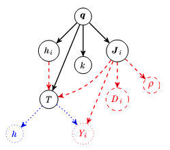
Example DAG for diffusive flux — Fig. 1.1 Example dependency graph for the calculation of the enthalpy diffusive flux. Solid lines are direct dependencies whereas dashed and dotted lines are dependencies discovered by following out-edges and recursively adding Expressions to the graph.

When compared to more “traditional” programming model of multiphysics environment, the Expression system offers a more algorithmically flexible approach by deducing data dependency of various models from the assembled graph (such as the one shown in Fig. 1.1); this eliminates the need for the application programmer to specify any complex logic for specific physics models and offers a generic method for generating an assembly routine for arbitrarily complex multiphysics simulations.

1.3.2. General Naming Convention

Due to the dynamic nature of fields, variables and expressions in Aria a consistent naming convention must be used for sanity sake. This section describes the format of string-names of Aria Expressions. These string forms are used for input and output only; Aria has more efficient internal structures for referencing Expressions. The general format of Aria’s string-based naming conventions for expression is as follows:

[<OPERATOR>_][<MATERIAL_PHASE>_]<NAME>[_<SUBINDEX>][_<PHASE>][_<COMPONENT>]

In the above syntax, square quantities within square brackets are optional. Common values for the <NAME> field include degrees of freedom (such as VELOCITY, TEMPERATURE, etc.) and material properties (VISCOSITY, DENSITY, etc.). A subset of common valid values for <OPERATOR> are listed in Table Table 1.1.

Table 1.1 Commonly used values for `<OPERATOR>` prefix
Operator	Description
(none)	“No-Op”, no-operator, Gauss point value
`DT`	Time derivative
`GRAD`	Gradient
`DIV`	Divergence
`DET`	Determinant of a second order tensor
`DETJ`	Determinant of the Jacobian of transformation for volume elements
`SURFACE_DETJ`	Determinant of the Jacobian of transformation for surface elements
`REF_FRAME`	“No-Op” in the undeformed reference frame
`GRAD_REF_FRAME`	Gradient in the undeformed reference frame
`OLD`	“No-Op” at previous time step
`REALLY_OLD`	“No-Op” at previous n-2 time step (for second order integrators)
`GRAD_OLD`	Gradient at the previous step
`DIV_OLD`	Divergence at the previous time step

The parameter <SUBINDEX> is used to designate multiple instances of a single field, and is typically used for species equations. All integer values are valid subindex values, but it’s best to use values $\geq 1$ .

The <PHASE> field is used to delineate between two phases separated by a level set interface; some fields are present in “all phases”, while others (such as material properties) depend on which phase is being referred to. Table Table 1.2 list valid values for this identifier:

Table 1.2 Valid values of the `<PHASE>` suffix
Phase	Description
(none)	Field is present in all phases
`A`	Phase A material
`B`	Phase B material
`C`	Phase C material

The <MATERIAL_PHASE> field is used to delineate between physical phases (e.g. solid, liquid, gas); some fields are present in “no material phase”, while others depend on which phase is being referred to. Table Table 1.3 list valid values for this identifier:

Table 1.3 Valid values of the `<MATERIAL_PHASE>` prefix
Phase	Description
(none)	Field is present in all phases (`NO_MATERIAL_PHASE`)
`LIQUID_PHASE`	Liquid phase material
`GAS_PHASE`	Gas phase material
`SOLID_PHASE`	Solid phase material
`WETTING_PHASE`	The wetting phase (e.g. liquid, less common)
`NONWETTING_PHASE`	The non-wetting phase (e.g. gas, less common)

Lastly, the COMPONENT field describes a component of either a vector or tensor field; valid values are listed in Table Table 1.4

Table 1.4 Commonly used component values for `<COMPONENT>` suffix
Component	Description
(none)	No specified component
`X`	First vector component
`Y`	Second vector component
`Z`	Third vector component
`XX`	(1,1) 2-tensor component (default: 0)
`XY`	(1,2) 2-tensor component (default: 0)
`XZ`	(1,3) 2-tensor component (default: 0)
`YX`	(2,1) 2-tensor component (default: 0)
`YY`	(2,2) 2-tensor component (default: 0)
`YZ`	(2,3) 2-tensor component (default: 0)
`ZX`	(3,1) 2-tensor component (default: 0)
`ZY`	(3,2) 2-tensor component (default: 0)
`ZZ`	(3,3) 2-tensor component (default: 0)

Understanding these components can help the user understand how to postprocess various quantities in their models; for example, postprocessing a quantity within a liquid phase material can be done with:

postprocess value of expression TEMPERATURE of Li+ in LIQUID_PHASE on all_blocks as foo

Note that in place of mangling the string, most line commands support the syntax…

[Quantity] [(Of|Species|Subindex) (SpeciesName)] [(In|Material_Phase) (MaterialPhaseName)] [(LevelSet_Phase|LS) (A|B|C)]

1.3.3. Equation-specific Naming Convention

String names of Aria equations also have similar restrictions posed in General Naming Convention. These formats are used for input and output only; Aria has an internal structure for referencing specific equations. Equation names follow the below format:

<EQUATION_NAME>[_<SUBINDEX>][_<PHASE>][_<COMPONENT>]

Again, values within square brackets are optional. Some valid values for <EQUATION_NAME> include MOMENTUM, ENERGY, SPECIES, LEVEL_SET etc. The <SUBINDEX>, <PHASE> and <COMPONENT> values are the same as those described in General Naming Convention.

1.3.4. Internal Field Definition

Internally, Aria contains an internal naming scheme for fields to facilitate their algorithmic usage. In most cases this naming convention will be <usage>->field_name where <usage> categorizes its internal usage. From a user perspective the <usage> category will be solution and as an example the voltage solution is internally known as solution->voltage. Application output is managed independent of the application thus output requests must correspond to the internal code Field names rather than the Field name stated in the previous section.

Note that some fields are stated- meaning that Aria retains their value at various time points. Valid names for these states are

Table 1.5 Field States
Component	Description
`NONE`	Corresponds to a field without state (only latest value)
`NEW`/`NP1`	Corresponds to the field value at the `NEW` time
`OLD`/`N`	Corresponds to the field value at the `OLD` time
`NM[X]`	Corresponds to the field value at `N-X`th old time for some integer X