5.1.3. Convective Flux BCs

This tutorial builds on the prior Materials and Flux BCs tutorial and shows how to add a convective flux boundary condition. This module has also been recorded in prior trainings and is available here or in the player below.

5.1.3.1. Problem Files

The files required for this tutorial can be downloaded here, or found at $SIERRA100/TF/Aria (where SIERRA100=/projects/sierra100 in a CEE environment, or your Sierra test distribution otherwise).

Aria input file

Mesh file

Training slides

5.1.3.2. Problem Domain/Mesh

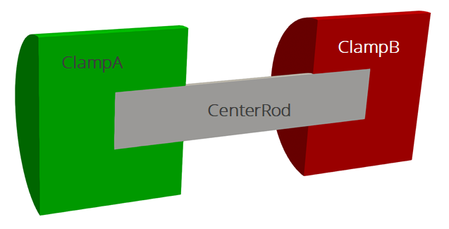
The geometry we will use for this tutorial is the same as the one used Basic Heat Conduction. It consists of three cylinders making a dumbbell shape, with three separate named blocks (ClampA, ClampB, and CenterRod). Blocks (volumetric sections in the mesh) are used in Aria to define different material properties, and can also be used to run post-processors on.

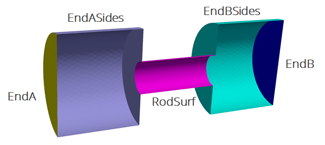
The problem also includes five separate named sidesets (EndA, EndB, EndASides, EndBSides, and RodSurf) applied on different surfaces of the mesh. Sidesets in aria are used to apply boundary conditions or do surface post-processing. Any surface not covered by a sideset will be treated as adiabatic, as will any sideset with no boundary condition applied to it.

The mesh file needed for this tutorial can be downloaded here, or it can be generated manually using the Cubit journal file shown in the Basic Heat Conduction tutorial.

5.1.3.3. Convection in Aria

Convection is when a solid exchanges energy with a moving fluid. When the fluid motion is externally driven, this is referred to as forced convection. When the fluid motion is driven by buoyancy from heating or cooling it is referred to as natural convection. There are a variety of ways to handle convection in Aria, described in broad terms below:

Pre-Computed Convection Coefficient: There are a wide variety of correlations available in the literature for estimating a convection coefficient for different geometries and fluid properties. When a convection coefficient can be calculated a priori one can use a simple flux model where $q = h(T - T_{ref})$ . In this case, $h$ and $T_{ref}$ are prescribed by the user as constants or simple functions.
Bulk Node + Correlation: A slightly more advanced option is to use a bulk node to solve an energy equation for the fluid along with a convection correlation from the built-in library.
Advective Bar + Correlation: This approach solves a 1D fluid flow equation along an advective bar which allows variation in temperature in both time and space. Coupled with a convection correlation from the built-in library this provides a way to model convection for simple flows.
Full CFD Solve: The most accurate, and most expensive approach is to do a full CFD solve for non-isothermal flow outside the object. This is often done using a coupled Fuego-Aria simulation.

This tutorial will use the pre-computed convection coefficient approach to add convection to the outer surfaces of the dumbbell geometry.

5.1.3.4. Adding a Convection BC

Scope: Aria Region

We will replace the variable flux we used for EndB from the last example with a constant.

BC Dirichlet for temperature on EndA = constant value = 300 # K
BC Flux for Energy on EndB = Constant value = -5e4

Next, we will create a mesh group to make applying the convection boundary conditions easier. The mesh group clamp_conv consists of two sidesets, and lets us apply boundary conditions to the mesh group instead of the individual sidesets.

Mesh Group clamp_conv = EndASides EndBSides

BC Flux for Energy on clamp_conv = Generalized_Nat_Conv H=5 T_ref=250
BC Flux for Energy on RodSurf = Generalized_Nat_Conv H=10 T_ref=250

Since we are applying constant values for $h$ and $T_{ref}$ we can use the Generalized_Nat_Conv boundary condition.

5.1.3.5. Post-process Flux

Scope: Aria Region

To see how much heat is lost due to convection, we will add some new postprocessors on the surfaces where we applied the convection boundary condition.

Postprocess integrated_flux of equation energy on clamp_conv as ClampConvLoss
Postprocess integrated_flux of equation energy on RodSurf as RodConvLoss

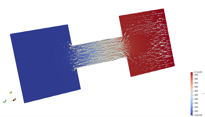
We can also add some post-processed fields to show the heat flux vector ( $-k\nabla T$ ) and the flux field on the RodSurf sideset.

Postprocess value of expression heat_conduction on all_blocks as HeatFlux
Postprocess value of expression energy_flux on RodSurf as ConvFlux

We have now created two new global variables (ClampConvLoss and RodConvLoss) and two nodal fields (HeatFlux and ConvFlux). To be able to see these fields, we need to also add them to the results output block.

Begin Results Output AriaOutput
    Title Aria: Transient Training Model
    Database Name = heat_cond.e
    At Step 0 Interval = 5
    Nodal Variables = Solution->Temperature as T
    Nodal Variables = ConvFlux
    Nodal Variables = HeatFlux

    Global Variables = FluxA
    Global Variables = FluxB
    Global Variables = ClampConvLoss
    Global Variables = RodConvLoss
End

5.1.3.6. Running Aria

Once you have finished setting up the input file, you are ready to run Aria. From a CEE unix environment, you can load the sierra module to access the latest release of Aria to run it on your local machine. To run it on 4 processors, you could use

$ module load sierra
$ launch -n 4 aria -i heat_cond_session2.i

5.1.3.7. Viewing the Results

From a CEE unix environment with graphics, you can launch paraview using

$ module load viz
$ paraview heat_cond.e.4.0

Or if you have installed Paraview locally, you can launch it and select the exodus file from the appropriate file opening menu.

Once you have loaded it, you need to select which variables to show then click Apply.

To show the convective flux field (ConvFlux) on the center rod, you can

Go to the last time step

Select the ConvFlux variable to show

Rescale the color scale if needed

The result shows how the flux varies across the center rod

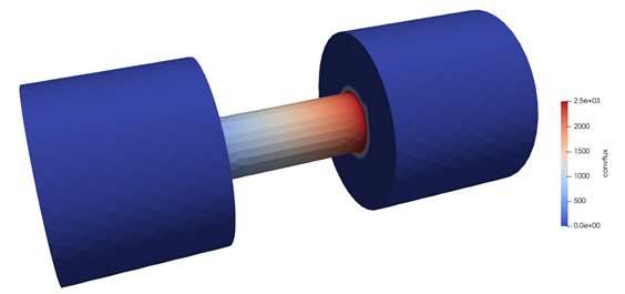
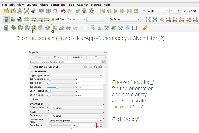
To view the heat flux vector through the center of the domain, you can

Slice the domain and click Apply

Create a Glyph filter

Choose HeatFlux for the orientation and scale array and set a scale factor of 1e-7

Click Apply