6.7.3. Expression Flux Limitations
6.7.3.1. Explanation
An expression flux postprocessor is often used for postprocessing on internal surfaces. Depending on the resolution and geometry a problem, one might find that the results from these postprocessors inaccurate. The root issue comes from the fact that Aria uses a finite element approximation. As opposed to a control-volume approach, a finite element approach does not generally guarantee equality of flux along element boundary. Within these elements, the gradient is recovered only up to a given order. Since expression flux postprocessors use the element’s gradient operator they are subject to these discretization errors.
To demonstrate this, consider the following example of two Quad4 elements sharing a face. For the linear function  , the elements can exactly recover the field solution and its constant gradient.
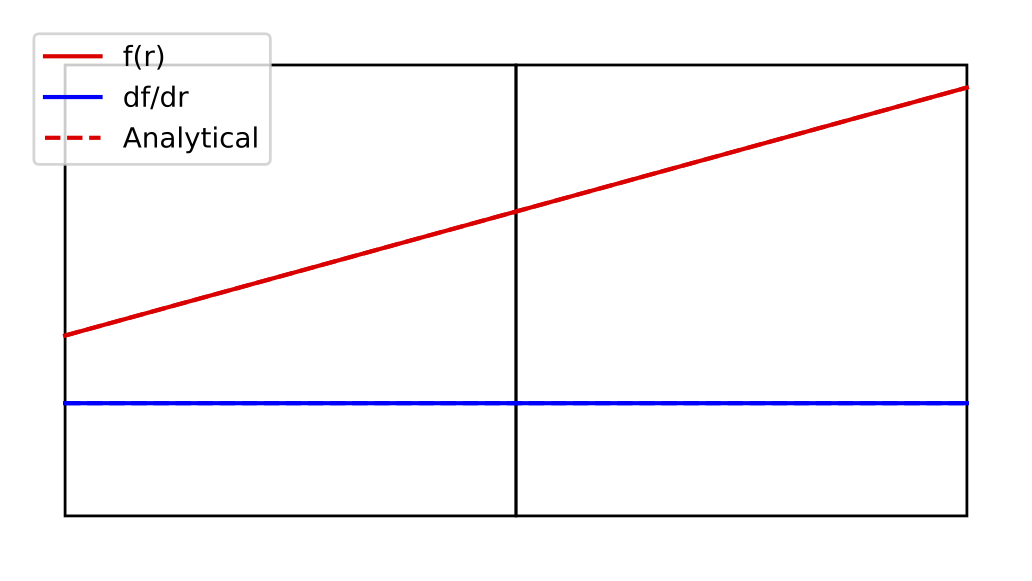
Fig. 6.3 Interpolated function and gradient for linear function
For the cubic function  on the other hand, the recovered gradient is not exact
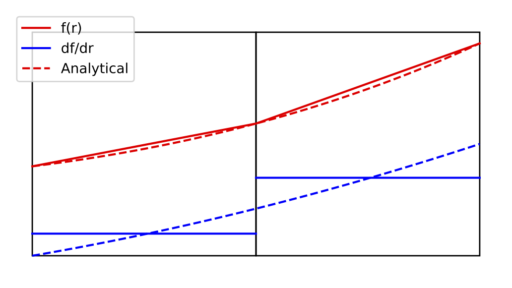
Fig. 6.4 Interpolated function and gradient for cubic function
As an example of the implication of this, consider the following domain
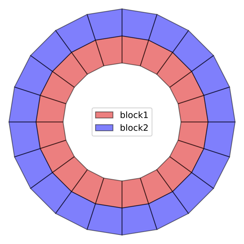
Fig. 6.5 Convergence study domain
In this study, the elements are shrunk to maintain the same aspect ratios with increasing resolution along the circumferential direction. The following quantities are calculated over the shared internal surface  at each resolution and included in the convergence plot below
- Circumference

- Radius

- Flux
 where the gradient of
  is evaluated using the element’s gradient operator
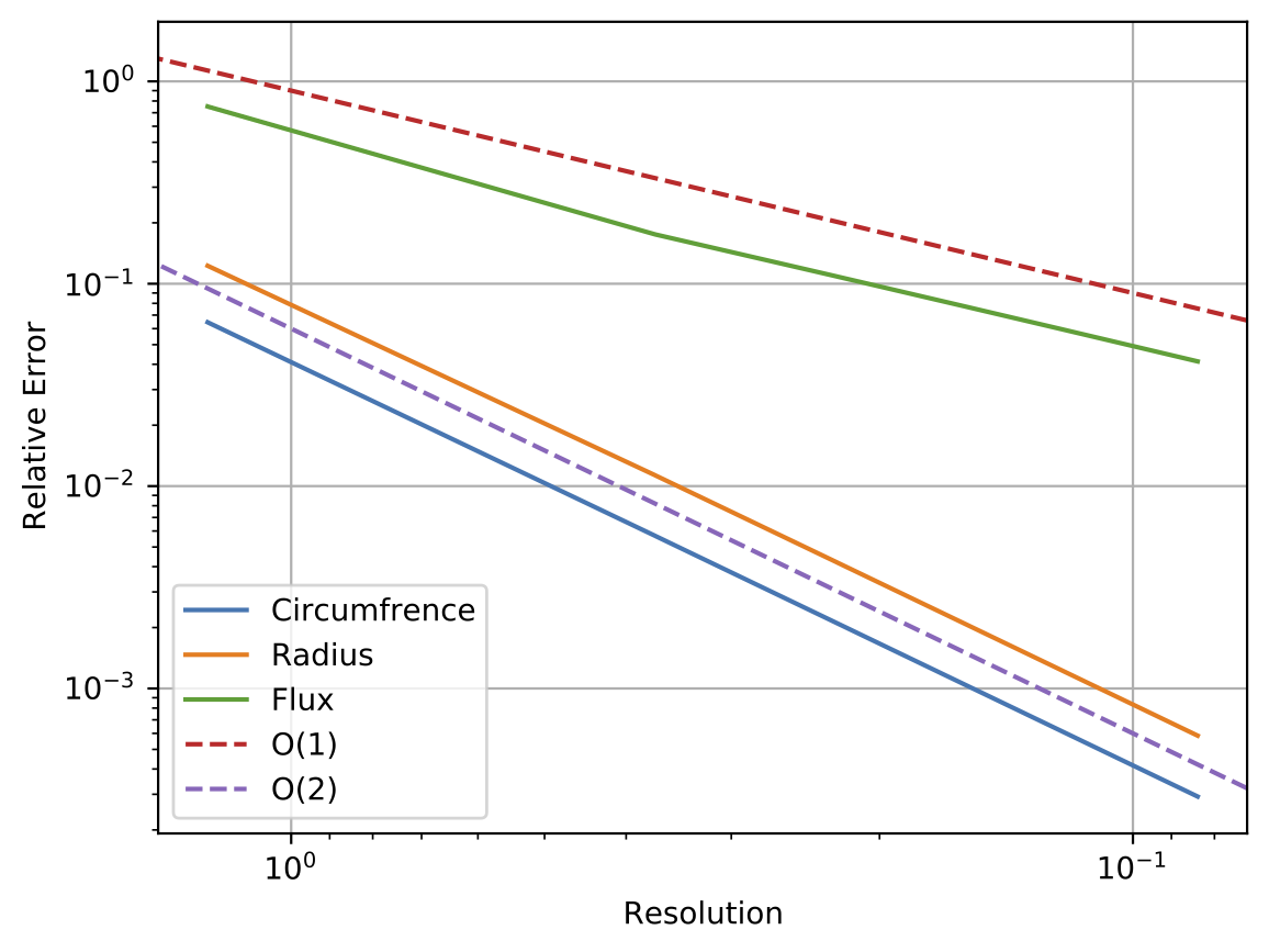
Fig. 6.6 Convergence study
As is expected, both the radius and circumference converge with O(2) with the linear elements used. Even for this simple geometry, though, the initial error of the flux term is a decade higher than that of the solution field. The convergence is also O(1) for the gradient-based term, as opposed to the solution field operations converging with O(2). This demonstration highlights why one might need to refine much more than is necessary to attain the proper finite element solution when using shape function gradients for postprocessing.
6.7.3.2. Solutions
The following section lists the possible solutions that can be taken, listed in order of their ease of implementing.
- Not on Internal surface? Replace with residual flux postprocessor.
If it possible to isolate the flux component of a term in a residual-flux postprocessor, this will always be the easiest way. For example for some
external_surface, one should postprocess the flux term separately and feed that into the remainder of the calculation e.g.# instead of using HEAT_CONDUCTION expression postprocess integrated_flux of vector_string_function \$ f_x = "HEAT_CONDUCTION_X * density" \$ f_y = "HEAT_CONDUCTION_Y * density" \$ f_z = "HEAT_CONDUCTION_Z * density" \$ on external_surface as foo_w_expr #postprocess the flux then feed it into an expression postprocess FLUX_SCALAR_FIELD of equation energy on external_surface as energy_flux postprocess integral of function "energy_flux * density" on external_surface as foo_w_residual_flux
- Average flux over both touching extents.
For some
internal_surfacetouching both blocks 1 and 2, performing the average over both touching extents will achieve a closer approximation since it averages the gradient contributions of both elements. As was demonstrated above, the average between the two elements will approach the true value at the face more quickly than each element’s values. Note that one of the terms must have a sign flipped so that the opposing normal directions do not cancel out.postprocess integrated_flux of expression HEAT_CONDUCTION on internal_surface touching block_1 as heat_flux_b1 postprocess integrated_flux of expression HEAT_CONDUCTION on internal_surface touching block_2 as heat_flux_b2 postprocess global_function "(heat_flux_b1 - heat_flux_b2)/2" as heat_flux
- Refine mesh either globally or locally.
If this term still is found to be too far off, refining the mesh can help. One option here is to locally refine the mesh along the surface of interest in the mesh generation software. If this portion of the mesh has a high gradient, adaptivity can be enabled in order to locally refine the interface using e.g.
# Scope: Sierra
Begin Recovery Indicator recover_ind
  Store In indicator_field
  Use Function solution->temperature
  Recover gradient
End
Begin Percent Of Max Marker max_mark
  Store In marker_field
  Use Element Field indicator_field
  Percent Of Max To Refine Above 80
  Percent Of Max To Coarsen Below 10
  Maximum Refinement Level 5
End
...
Begin Transient time_stepping_block
  advance AriaRegion

  IndicateMarkAdapt AriaRegion Using recover_ind max_mark \$
    when "transient_time_stepping_block.CURRENT_STEP % 5 == 0"
End Transient
- Extract net flux from volume integrated quantities.
Finally if the mesh cannot be refined, one could keep track of the net generation of the equation and subtract off any sources to get the net flux out of the body. Since this approach avoids any gradient-based quantities, it will give a notably more accurate result.
postprocess integral of function "dt_temperature*specific_heat*density" on each_block as net_energy_gen
postprocess integral of expression energy_source on each_block as internal_energy_src

# Calculate the component of energy generation that came from fluxes
postprocess global_function "net_energy_gen_block_1 - internal_energy_src_block_1" as net_energy_flux_block_1
postprocess global_function "net_energy_gen_block_2 - internal_energy_src_block_2" as net_energy_flux_block_2
postprocess global_function "net_energy_gen_block_3 - internal_energy_src_block_3" as net_energy_flux_block_3
- Subtract the component due to external flux via residual-flux postprocessor.
If one is interested in the relative contributions of internal and external fluxes, a residual flux postprocessor can be run over the external surfaces of each block. Again since these postprocessors use the residual of the true equations solved, they will not be subject to the discretization errors discussed above
# Find the external component of the fluxes on each body
postprocess integrated_flux of equation energy on b1_ext_surf as net_ext_flux_block_1
postprocess integrated_flux of equation energy on b2_ext_surf as net_ext_flux_block_2
postprocess integrated_flux of equation energy on b3_ext_surf as net_ext_flux_block_3

# What remains is the net internal fluxes
postprocess global_function "net_energy_flux_block_1 - net_ext_flux_block_1" as net_int_flux_block_1
postprocess global_function "net_energy_flux_block_2 - net_ext_flux_block_2" as net_int_flux_block_2
postprocess global_function "net_energy_flux_block_3 - net_ext_flux_block_3" as net_int_flux_block_3
- Postprocess relative internal flux across blocks
Finally, if one wants to know the relative internal flux between each block, the
net_int_fluxcan be written to a a heartbeat file. The relative internal fluxes can then be back-calculated in postprocessing of the results e.g.import numpy as np # 1->2, 2->3, 3->1 connectivity = np.array([ [ 1, 0,-1], #block 1 [-1, 1, 0], #block 2 [ 0,-1, 1], #block 3 ]) net_int_flux = np.array([ net_int_flux_block_1, net_int_flux_block_2, net_int_flux_block_3, ]) # Overwrite row and fix mean internal flux at zero net_int_flux[-1] = 0 connectivity[-1,:] = 1 fluxComps = np.linalg.solve(connectivity, net_int_flux) rel_internal_flux_1to2 = fluxComps[0] rel_internal_flux_2to3 = fluxComps[1] rel_internal_flux_3to1 = fluxComps[2]
Note that the original linear system is singular (any solution +C satisfies the net flux condition), we must override one of the rows and the solution is only the RELATIVE flux between the blocks.