3.2.4.19. Level Set

The level set method resolves evolving interfaces between multiple phases within a domain; this is done by tracking a smooth signed distance function $\levelSet$ over the domain that indicates the closest distance to the interface at any point. An example of a $\levelSet$ function is given for a 2D circular interface ( $\levelSet = \sqrt{x^{2} + y^{2}} - 1$ ), is shown in Fig. 3.2

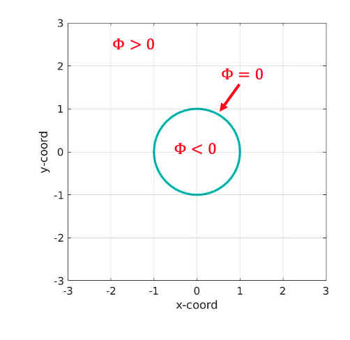
Fig. 3.2 Schematic of 2D circular interface using a signed distance function

As seen in Fig. 3.2, values where $\levelSet < 0$ indicate one phase, and $\levelSet > 0$ indicates another; the interface separating the two phases is represented by the $\levelSet = 0$ isocontour. Geometric parameters such as the interface normal $\levelSetNormal$ and curvature $\levelSetCurv$ can be calculated directly from $\levelSet$ since it is a smooth function:

(3.88) $\levelSetNormal = \frac{\nabla \levelSet}{\|\nabla \levelSet\|}, \; \; \; \; \levelSetCurv = \nabla \cdot \levelSetNormal$

An important property of $\levelSet$ is that it remains a signed distance function; this ensures that the computations in (3.88) are accurate. This property is enforced by ensuring the norm of the gradient of $\levelSet$ is equal to 1:

(3.89) $\| \nabla \levelSet \| = 1$

The variable $\levelSet$ is typically advected with the fluid velocity $\v$ , which is obtained from the solution of (3.22):

(3.90) $\pt{\levelSet} + \v \cdot \nabla \levelSet = 0$

In general, Eq. (3.90) does not satisfy the property posed by Eq. (3.89). An additional redistancing operation must be performed throughout the simulation, which will be discussed in Level Set/CDFEM. Aria allows the user to define generic sources $S_{V}$ to model any sinks/production rates into the level set field, thus (3.90) is modified to:

(3.91) $\underbrace{\pt{\levelSet}}_\mathrm{MASS} + \underbrace{\v \cdot \nabla \levelSet}_\mathrm{ADV} - \underbrace{S_{V}}_\mathrm{SRC} = 0$