 |
Home > Mesh Generation > adaptivity and sizing functions > Exodus II-based Field Function
|
Cubit 16.02 User Documentation
The ability to specify the size of elements based on a general field function is also available in CUBIT. With this capability, the desired element size can be determined using a field variable read from a time-dependent variable in an Exodus II file. Both quadrilateral and triangle elements are supported for surfaces, and both tetrahedral and hexahedral elements are supported for volumes.
A field function is a time-dependent variable in an Exodus II file. Either node-based or element-based variables may be used. Currently, field functions are imported from element and node-based Exodus II data. The mesh block containing the corresponding elements must be imported along with the field function data.
Exodus variable-based adaptive meshing is accomplished in CUBIT in several steps:
Importing a field function, and normalizing that function are done in two separate steps to allow renormalization. The following command is used to read in a mesh for the field function:
Import Sizing Function '<exodusII_filename>' Block <block_id> Variable `<variable_name>' [Time <time_val> | Step <step> | Last] [Deformed]
The block_id is the element block to be read, which can be a single block id or the word all. The variable_name is an Exodus time-dependent variable name (either element-based or nodal-based) which values are used to drive the mesh size. The timestep for the time-dependent variable can be specified as a time with a value, as a step with an index or Last to use the last timestep in the file. The Deformed keyword indicates whether to read the deformed field function mesh, which should align with the geometry being meshed and needs to be accounted for in the field function data. (For information on creating deformed geometry from EXODUSII data, see Importing 2D EXODUSII Files and Importing EXODUSII Files) .
Note that when a field function is read in, the mesh is stored in the background, and therefore the geometry is not considered meshed. Also note that if deformation is not being modeled, the geometry should be in the same state as it was when that mesh was written (see Importing a Mesh for more details on importing meshes).
Once the field function has been read in, it can be normalized before being used to generate a mesh. The normalization parameters (Min_size and Max_size) are specified in the same command that is used to specify the sizing function type for the surface or volume. The syntax of these commands are:
Surface <id> Sizing Function Type Exodus [Min_size <min_val> Max_size <max_val> Log_Map Inverse_Map Scale_Mesh_Multiplier <value>]
Volume <id> Sizing Function Type Exodus [Min_size <min_val> Max_size <max_val> Log_Map Inverse_Map Scale_Mesh_Multiplier <value>]
If normalization parameters are specified, the field function is normalized so that its range falls between the minimum and maximum values input. If an element-based variable is used for the sizing function each node is assigned a value that is the average of variables on all connected elements. Nodal variables are used directly.
The Log_Map option maps the range so that it is logarithmic, base 10.
Inverse_Map flips the mapping so that smaller and larger values in the mapping generate larger and smaller elements respectively. See figure 1 below.
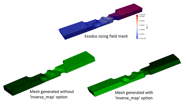
Figure 1. Effect of 'inverse_map' option
Scale_Mesh_Multiplier scales the size that the field data ultimately yields.
After the sizing function normalization, the geometry may be meshed using the normal meshing command.
For example, the left image in Figure 2 depicts a plastic strain metric which was generated by PRONTO-3D [Taylor, 89] a transient solid dynamics solver, and recorded into an ExodusII data file. When the file is read back into CUBIT, the paving algorithm is driven by the function values at the original node locations, resulting in an adaptively generated mesh [Attaway, 93]. The right image in Figure 1 depicts the resulting mesh from this plastic strain objective function.
Figure 2. Plastic strain metric and the adaptively generated mesh
While adaptively meshing a surface using a field function, the curves will be meshed using the Exodus II information. To override this, curves may have their meshing scheme set to equal or some other desired scheme. While adaptively meshing a volume using a field function, the surfaces and curves will be meshed using the Exodus II information. To override this for a surface, one can set the sizing function to "none" for that surface.